by Prasad Raghavendra (Simons Institute)

Another semester of remote activities at the Simons Institute draws to a close. In our second semester of remote operations, many of the quirks of running programs online had been ironed out. But pesky challenges such as participants being in different time zones remained. To cope with these, the programs spread their workshop activities throughout the semester. Not only did this help with the time zones, but it helped keep up the intensity all through the semester.

One hopes that the Institute will never need to organize a remote semester again. At the end of June, we are excited to host the Summer Cluster in Quantum Computation, our first in-person activity since COVID-19 hit. By all expectations, the programs in the fall will likely be fairly close to the normal that we have all been longing for.

In fact, it looks like the Institute will be buzzing with activities in the fall, even more than it used to be, as if that were possible. In a few months, the Institute will welcome more than 40 talented young researchers as postdoctoral researchers and program fellows. They cover the whole gamut of areas, ranging from complexity theory and algorithms to quantum computation and machine learning.

As we settle into a different normal again, one wonders what this new normal will look like a few years from now. In particular, what aspects of this COVID era will continue to stay with us theorists, say, five years from now? Will we have online conferences and workshops? Will meeting anyone from anywhere seem as easy as it does now? How often will a speaker be physically present at our seminars? Only time will tell.

Solving linear systems faster
The ACM SODA conference held virtually in January featured a breakthrough result in algorithms for one of the oldest computational problems — namely, solving a system of linear equations. Richard Peng and Santosh Vempala exhibited a new algorithm to solve sparse linear systems that beats matrix multiplication, in certain regimes of parameters.

Needless to say, the problem of solving a system of linear equations is fundamental to a wide variety of applications all across science and engineering. Broadly, there are two families of approaches to solving a linear system. First, we have the so-called direct methods such as Gaussian elimination, Cramer’s rule or more sophisticated algorithms that reduce solving linear systems to matrix multiplication. These algorithms incur O(n²) space, which can be quite prohibitive for sparse linear systems. However, these algorithms have a mild polylogarithmic dependence on numerical parameters such as condition number. The condition number of a linear system Ax = b is the ratio of the largest to the smallest eigenvalue of matrix A.

The second family of algorithms consists of iterative algorithms such as gradient descent that minimize the least squares error. In particular, these algorithms maintain an approximate solution which they improve by updates akin to gradient descent. Iterative methods have little space overhead (roughly O(n) space) and therefore are widely used for solving large, sparse linear systems that arise in scientific computing. Furthermore, these algorithms are naturally suited to producing approximate solutions of desired accuracy in floating-point arithmetic. Perhaps the most famous iterative method is the conjugate gradient algorithm from the 1950s. The conjugate gradient algorithm runs in O(n • nnz) time in unbounded precision arithmetic, where n is the number of variables and nnz is the number of nonzero entries in the matrix A corresponding to linear system Ax = b.

Unfortunately, the run-time of iterative methods depends polynomially on the condition number. In particular, consider a linear system Ax = b, where A has about O(n) nonzeros and a condition number, say n¹⁰. Iterative methods yield a large polynomial run-time that is of no value here.

The number of iterations of algorithms such as gradient descent can be improved by preconditioning the domain — i.e., suitably rescaling the domain. However, preconditioning the domain is not always easy in general. For certain special classes of linear systems, one can exploit the combinatorial structure of the matrix A to precondition the linear system efficiently. The most influential example of such a special case is that of Laplacian linear systems. Inspired by heuristic approaches from scientific computing, Spielman and Teng in a tour de force exhibited the first near-linear time algorithms for Laplacian systems in 2004. The rest is history. We now have Laplacian system solvers that are faster than sorting algorithms, and these solvers have been used as building blocks to solve other problems, such as maximum flow, faster.

There have been generalizations, such as finite-element matrices and directed graphs, that also admit near-linear time algorithms. Yet, for general sparse linear systems, these iterative algorithms fail, and the best algorithms were all based on reduction to fast matrix multiplication. In fact, it was widely hypothesized that solving general sparse linear systems is as hard as general matrix multiplication.

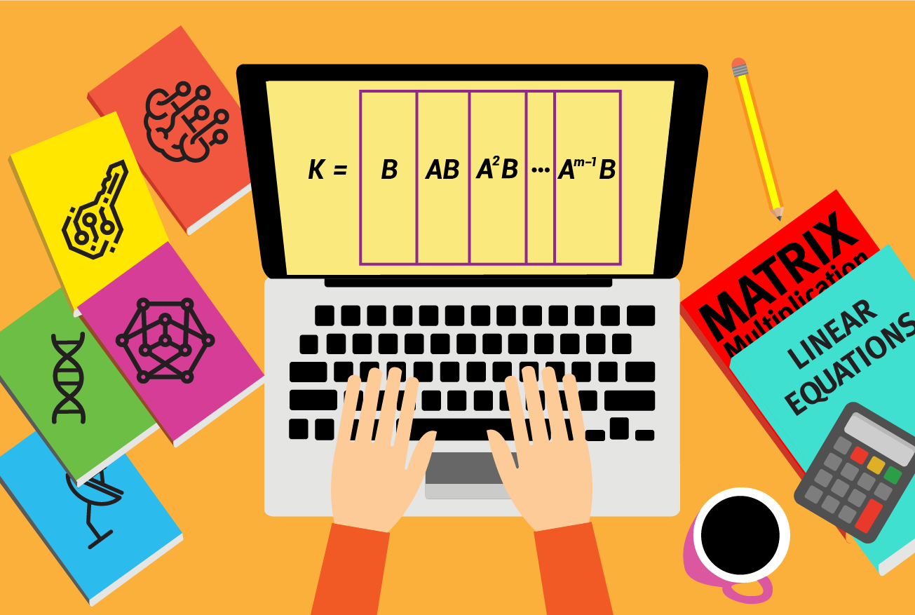
The breakthrough work of Peng and Vempala exhibits an algorithm that refutes this strong hardness assumption. In particular, for sparse matrices with O(n) entries and a polynomial condition number, this is the first algorithm that beats matrix multiplication run-time. As is often the case, the algorithm is a result of tying together ideas from two distinct algorithmic threads, namely direct and iterative algorithms. Specifically, the algorithm constructs block Krylov subspaces inspired by the conjugate gradient algorithm, and solves the associated linear systems with block Hankel structure, while ensuring that the numbers used do not blow up.