We no longer actively maintain this blog. Please subscribe to our newsletter!
This blog has sunsetted
Reply
We no longer actively maintain this blog. Please subscribe to our newsletter!

by Nikhil Srivastava (senior scientist, Simons Institute for the Theory of Computing)
Expanders are sparse and yet highly connected graphs. They appear in many areas of theory: pseudorandomness, error-correcting codes, graph algorithms, Markov chain mixing, and more. I want to tell you about two results, proven in the last few months, that constitute a phase transition in our understanding of expanders.
Random graphs are Ramanujan with 69% probability
One way to quantify the expansion of a graph is via its adjacency spectrum. A \(d\)-regular graph is called Ramanujan if its nontrivial (i.e., other than \(d\)) adjacency eigenvalues are bounded in absolute value by \(2\sqrt{d-1}\). Alon and Boppana showed in 1986 that no infinite sequence of graphs can have nontrivial eigenvalues concentrated on a smaller interval, so Ramanujan graphs may be viewed as optimal spectral expanders as a function of \(d\).
The most important result about Ramanujan graphs is that they exist. Motivated by the Alon-Boppana bound, Lubotzky, Phillips, and Sarnak and independently Margulis famously constructed infinite sequences of Ramanujan graphs whenever \(d = p + 1\) for a prime number \(p\) in 1988. This is a gift that keeps on giving, as we will see below, albeit one whose proof very few of its recipients understand.
Until December 2024, that was the only known proof of the existence of Ramanujan graphs. Two results came close: Friedman’s theorem (and its improvements) that random \(d\)-regular graphs are almost Ramanujan with high probability, and the existence and construction of bipartite Ramanujan graphs (which are allowed to have an extra eigenvalue of -\(d\)) for all \(d\) via the interlacing families method. It remained mysterious whether the existence of Ramanujan graphs was a precious miracle or the consequence of some robust phenomena.
Huang, McKenzie, and Yau have shown that a random \(d\)-regular graph on \(N\) vertices is Ramanujan with probability approaching 69% as \(N\) \(\rightarrow\) \(\infty\). The fact that this probability does not approach 0 or 1 is strange in the context of the probabilistic method (as reflected in a bet of Noga Alon and Peter Sarnak) and rules out typical proof techniques like concentration inequalities. But it was anticipated about 20 years ago in a different context: the universality phenomenon in random matrix theory.
Universality is like the central limit theorem. It predicts (among other things) that the distribution of the top eigenvalue of an \(N\)\(\times\)\(N\) real symmetric random matrix with independent normalized entries should converge (after appropriate scaling) to a universal law, regardless of the details of the entries. That limit is the Tracy-Widom law, discovered in 1994. The TW law shows up in many contexts — as the top eigenvalue of Gaussian and Wigner random matrices, as the distribution of the length of the longest increasing subsequence in random permutations, and as the distribution of fluctuations in liquid crystal droplets which can be seen in experiments. It is surprising to me that something so deeply embedded in nature was discovered only 30 years ago, though the proposal of universality in random matrix theory goes back to Wigner in the 1950s (in the context of spacings of eigenvalues rather than top eigenvalues, which he used to model the energy gaps of heavy nuclei).
Numerical experiments by Novikoff, Miller, and Sabelli from around 2004 suggested that the extreme nontrivial eigenvalues of random \(d\)-regular graphs should have asymptotically independent Tracy-Widom fluctuations (which are of scale \(N^{-2/3}\)) centered near \(\pm\)\(2\sqrt{d-1}\). Conceptually, this would mean that the edge eigenvalue fluctuations of random \(d\)-regular graphs behave like those of Gaussian orthogonal ensemble (GOE) matrices. This is subtle because the same is definitely not true for sparse Erdős-Rényi graphs, whose extreme eigenvalues are dominated by high-degree vertices. Proving this rigorously would immediately imply a constant probability of being Ramanujan, a proof combining both concentration and anticoncentration of the extreme eigenvalues.
This is what Huang, McKenzie, and Yau achieve. Their approach is a variant of the “local relaxation flow” strategy for proving universality results, introduced by Erdős, Schlein, and Yau in 2009 and refined in dozens of papers since then (see also this book). Letting \(A\) denote the adjacency matrix of a random \(d\)-regular graph on \(N\) vertices, the three steps in this strategy are:
Continue reading
by Nikhil Srivastava (senior scientist, Simons Institute for the Theory of Computing)
Some results mark the end of a long quest, whereas others open up new worlds for exploration. Then there are works that change our perspective and make the familiar unfamiliar once more. I am delighted to tell you about some recent developments of all three kinds.
Quantum Gibbs samplers
It seemed like everyone and their mother was talking about Gibbs samplers during the Simons Institute’s program on Quantum Algorithms, Complexity, and Fault Tolerance. The subject also had its very own one-day workshop. It made me wonder whether this is what it was like in the 1980s, before the first TCS results about efficient sampling via rapid mixing of MCMC came out.
A classical Gibbs distribution is a special kind of probability distribution that appears in statistical mechanics, machine learning, and other areas. For a spin system with \(n\) particles, it has pdf
\[p(x)\propto \exp(-\beta H(x)), x\in \{-1,1\}^n\]
where \(H(x)\) is a function prescribing the energy of a configuration \(x\), known as the Hamiltonian. Typically, the Hamiltonian is itself a sum of “local terms” that only depend on a constant number of spins each, modeling the locality of physical interactions. A good example to keep in mind is the Ising model. The reason for the exponential form of the Gibbs distribution is that it maximizes the entropy over all probability distributions having a prescribed average energy.
There is a highly successful theory of sampling from classical Gibbs distributions. In particular, there is a canonical Markov chain for doing this known as the Glauber dynamics. The transitions of the Glauber dynamics are as follows: pick a particle at random, look at its neighbors, and resample the spin of the particle from the correct conditional distribution given its neighbors. The reason this dynamics is easy to implement is that the Gibbs distribution of a local Hamiltonian has a lot of conditional independence in it; in particular, the distribution of a particle’s spin is conditionally independent of the rest of the spins given the spins of its neighbors, which is known as the Markov property. Thus, locality of the Hamiltonian translates to locality of the distribution, which further yields locality of the dynamics. This locality makes it easy to check that the Glauber dynamics has the correct stationary distribution by checking the detailed balance condition \(p(i)p_{ij} = p(j)p_{ji}\) where \(P=(p_{ij})\) is the transition matrix of the Markov chain.
Proving rapid mixing — i.e., that \[||P^t x-p||_1\rightarrow 0\] rapidly from any initial distribution \(x\) — is typically much harder. At this point, there is a huge arsenal of methods for doing it, including functional inequalities, coupling arguments, and, most recently, the theory of spectral independence and stochastic localization. A conceptually satisfying feature of this theory is that it is able to show that the computational thresholds for rapid mixing of Glauber dynamics are related to certain physical thresholds intrinsic to the Hamiltonian.
Let us now understand the quantum analogue of the above setup.
The theory community mourns the loss of Luca Trevisan. We hope that this page will serve as an enduring memorial to a brilliant scientist and expositor, and beloved friend and colleague. Please share your memories, roasts, and toasts in the comments.
Farewell to Luca
by Venkatesan Guruswami, Nikhil Srivastava, and Kristin Kane
We are heartbroken by the untimely loss of Luca Trevisan, who served as senior scientist at the Simons Institute from 2014 to 2019. Luca passed away on June 19 in Milan at the age of 52. His husband, Junce, was at his side along with a few other loved ones, notably our colleagues Alon Rosen and Salil Vadhan, who accompanied him in his last difficult months. Luca leaves behind a rich and diverse legacy of influential results, the Trevisan extractor being a masterpiece highlight.
An only child, Luca was born and raised in Rome, where as an adolescent he spent many long afternoons reading books about mathematics. He loved to cycle to Villa Ada or along the river Tiber, and was passionate about film — in particular Mel Brooks’s Young Frankenstein, and films by Monty Python and Woody Allen. In school, Luca earned the highest marks, but he was particularly precocious in mathematics. Luca’s lifelong friend Flavio Marchetti recalls, “I’ve often spoken about Luca with our high school mathematics teacher Daniela Crosti … and we joke about Luca’s questions, which frequently turned into extemporaneous original demonstrations in which he arrived at the answers by reasoning together with the class, without any advance preparation.”
As an undergraduate at Sapienza University in Rome, he became the first student to graduate from the department of information science. An article about the event in the Roman newspaper Il messaggero from July 20, 1993, sheds some light on Luca’s youthful personality. Luca’s mother, Giuseppina, described him as calm, disorganized, and not very well equipped to deal with practical matters. Friends remarked that he drove like a madman and was a danger to public safety, but had a great sense of humor.
After receiving his doctorate from Sapienza in 1997, Luca went on to postdoctoral positions at MIT and DIMACS. He then served on the faculty of Columbia, Berkeley, and Stanford, before taking a position as the Simons Institute’s senior scientist in 2014.
As senior scientist at the Simons Institute, Luca oversaw the Institute’s postdoctoral training program, mentoring a generation of rising stars in the field. He also spearheaded a research program on Pseudorandomness in Spring 2017 and brought several other successful research programs to the Institute through his outreach to potential organizers.
“There is no question that Luca significantly elevated the intellectual climate in the theory group at Berkeley,” remarks Simons Institute Founding Associate Director Alistair Sinclair, “and did so moreover with great humility and a disarming sense of humor. His ability to distill the essence of a huge range of mathematical ideas, and generously share his insights with others, through his blog and elsewhere, was a truly rare gift. It was a major coup for Berkeley to bring him back from Stanford as senior scientist at Simons. His advice and words of wisdom were invaluable during the endless rounds of decisions we faced in the early years of the Institute.”
In 2019, Luca returned to Italy to help launch the new Department of Computing Sciences at Bocconi University in Milan. At Bocconi, Luca held the Invernizzi Foundation Chair in Computer Science and cofounded and directed the two-year master of science in artificial intelligence, which was launched in Fall 2023.
Simons Institute Director Shafi Goldwasser recollects, “I overlapped with Luca at several stations along the way. I recall Luca as a young Italian postdoc who arrived at MIT, quiet and deep with an engaging smile, who surprised us one day with his extractor result while we were all occupied with PCPs. A few years later we had a pivotal conversation in a café in NYC when he was laboring over the decision to move to Berkeley; more than a decade passed before Luca welcomed me back to Berkeley, where he already was a senior scientist at the Simons Institute and his eloquent descriptions of ‘scientific pearls’ that arose in the programs were second to none. And finally a few months ago before any notion of illness was in the air, at dinner in Milan at the truly beautiful home he built for himself and Junce. I cannot believe we shall not meet again someday, somewhere.”
In the course of his career, Luca made beautiful contributions across the theory of computing, spanning pseudorandomness, approximate optimization and PCPs, property testing, spectral algorithms, and, in recent years, distributed computing. Luca’s PhD research in the mid-1990s focused on approximability and included two very elegant non-approximability results: one showing that the doubly exponential dependence on the dimension of the approximation schemes for Euclidean TSP was inherent, and another that provided a systematic LP-based framework to discover gap-preserving gadget reductions and argue their optimality. By the time he received his PhD, Luca had become an expert on the then rapidly evolving PCP literature. (Speaking of Luca’s PCP works, I (Venkat) was fortunate to coauthor my first paper in graduate school with Luca, which included a 3-query PCP with optimal soundness error.)
Among Luca’s varied contributions to PCPs is a line of work that culminated with PCPs with the best bang for the buck for queries made, asymptotically yielding an almost factor-two gain in soundness for each additional bit queried. The final paper in this series, from 2006, brought in tools from additive combinatorics like Gowers norms into the purview of TCS. Luca had a real knack for identifying directions in math with fruitful connections to complexity theory (and vice versa). As another example, he found two-way connections between dense model theorems that play a central role in the Green-Tao theorem on arbitrarily long arithmetic progressions in primes and the hard-core set theorem in complexity.
Luca was a true intellectual leader of our field. One way was of course through his many landmark theorems — for instance, his instant classic work connecting randomness extractors to pseudorandomness generators. Its underlying key insight, relating certain proofs in the computational world to information-theoretic counterparts, was a true gem, something so natural in hindsight yet never realized by the community. Another example is his more recent work generalizing Cheeger’s inequality to k-way cuts. These are the kind of results that will matter as long as our field exists. Reading their beautiful proofs, there is an inevitability about them that makes them hard to unsee.
Luca had an uncanny ability to quickly identify the significance and potential of a new direction when he saw one. He would comprehend the essence of the first paper on a topic at great depth, write a beautiful follow-up filled with insights that clarified and improved matters, and in turn inspire further follow-ups and progress. He did this repeatedly, on diverse topics, ranging from hardness amplification to Unique Games algorithms. This is best articulated in Luca’s own words in his blog post “On being second.”
Beyond his research prowess, Luca was a leader in another (more subtle) way, which is no less important. As a teacher and expositor, Luca awakened curiosity in others. In his many survey articles and lecture notes, he gave us the crispest expositions of many canonical results in theoretical computer science. His way of explaining was generous, making full use of his intellect but keeping it in the background. His writings made theoretical computer science seem approachable to me (Nikhil), as a graduate student outside one of the big theory groups. Both of us (Nikhil and Venkat) regularly benefited from Luca’s notes for our teaching — he had a gift for distilling advanced material in an engaging style perfectly tuned and packaged for lectures; in fact, we sometimes picked topics to lecture on because Luca had notes on them!
On his blog, in theory, in addition to his lecture notes, Luca also shared with us what he was learning. This included topics such as zeta functions, manifolds, and other objects not so familiar to the TCS audience. It was an invitation to expand our imagination, and a reminder that it’s okay to just learn something for its own sake. In person, Luca had a way of asking simple questions and then exploring them with clarity, devoid of any hint of competition or rush. Talking with him was a gentle invitation to wonder. He shared his questions and insights generously, and repeatedly went out of his way to collaborate with junior people, not even necessarily his students, including us. We doubt that our journey with Luca is unique. He represents what is best about our field: its openness and the generosity of its leaders. We hope that Luca’s way will forever remain alive in our community.
As a faculty member for over 25 years, Luca was a beloved mentor to many students. He both collaborated with them on influential results, and inspired them to grow as fearless researchers with their own ambitious agendas.
On a personal level, Luca was one of the out, gay theoretical computer scientists who have helped make this community a welcoming one for LGBTQIA+ researchers and students. He recounted his coming-out in 2000 in a characteristically humorous (and now legendary) blog post in honor of the Turing Centenary.
He was a fellow of the ACM, a member of the Italian National Academy of Science, and the recipient of the Oberwolfach Prize, a Sloan Research Fellowship, an NSF CAREER Award, and an ERC Advanced Grant. At the time of his passing, Luca was a member of the ACM A.M. Turing Award Committee.
Luca was a brilliant scientist and expositor, and unfailingly funny friend and colleague. His clarity and insight deepened our understanding, and advanced the frontiers of research in the theory of computing. Luca leaves behind an enduring scientific legacy. He will be sorely missed.

by Adam Becker (science communicator in residence, Spring 2023)
Think about the last time you faced a problem you couldn’t solve. Say it was something practical, something that seemed small — a leaky faucet, for example. There’s an exposed screw right on the top of the faucet handle, so you figure all you need to do is turn the faucet off as far as it will go, and then tighten that screw. So you try that, and it doesn’t work. You get a different screwdriver, a better fit for the screw, but you can’t get it to budge. You grab a wrench and take apart the faucet handle, and that doesn’t help much either — it turns out there’s far more under there than you’d expected, and you can barely put it back together again. You’re about to give up and call a plumber, but first you want to see whether you’re close. Maybe it really is easy to fix the problem, and you just need to know where to look. Or maybe it’s far more difficult than you think. So now you’re trying to solve a new problem, a meta-problem: instead of fixing the leaky faucet, you’re trying to figure out how hard it will be to fix the leaky faucet. You turn to the internet, and find that there are many different kinds of faucets and sinks, some of which are practically indistinguishable, and there are different reasons they can leak, unique to each type of sink. Simply determining the difficulty of fixing your leaky faucet is itself turning out to be more difficult than you expected.
Theoretical computer scientists have been facing their own version of this problem for decades. Many of the problems they ask are about complexity: How hard must a computer (really, an idealized version of one) work to perform a particular task? One such task, famous in the annals of both mathematics and computer science — theoretical computer science is where the two disciplines meet — is the traveling salesperson problem. Imagine a traveling salesperson, going from city to city. Starting from her home, she has a list of cities she must visit, and a map with the distances between those cities. Her budget limits the total distance she can travel to a certain maximum, so she’d like to find a route shorter than that maximum distance that allows her to visit each of the cities on her list, returning to her home city at the end. Given her list of cities and her budget, does such a route exist?
There is no known method for solving this problem quickly in a general way — a method that would work for all possible budgets and lists of cities that the salesperson might have. There are ways of doing it, but all of them take a large number of calculations relative to the number of cities on the list, and thus take a great deal of time, especially as the number of cities increases. In fact, the shortest such guaranteed method known for solving the traveling salesperson problem takes, in general, an exponentially larger amount of time as the number of cities on the list increases, because there’s no known way to do this that’s significantly faster than brute-forcing the problem by checking every possible route. Compare this with verifying a solution to the traveling salesperson problem: that’s easy. All you have to do is confirm that the solution does in fact visit every city once, and that the total distance of the route is shorter than the maximum allowed by the salesperson’s budget.
This property of the traveling salesperson problem — it seems like it can be solved in general only by a lengthy brute-force method, but it’s fast to verify a given solution — places it into a class of “computational complexity” known as NP. (This stands for “nondeterministic polynomial time,” and it’s not particularly important to understand that name in order to understand what’s going on here.) Compare this with a problem like determining whether the last entry on a list of numbers is the largest, for which there are known (and straightforward) methods that don’t scale exponentially with the length of the list. Such problems, which can be solved and verified quickly, are in a complexity class called P, a special subset of NP.
On the face of it, NP and P seem to be different; the traveling salesperson problem (TSP) can’t be solved quickly by any known method. But the trouble, for computer scientists, begins with those words “known method.” While nobody knows a fast way of solving a problem like the traveling salesperson problem, that doesn’t mean no such method exists. Finding such a method would show that TSP actually belongs in P. In fact, it would show more than that, because computer scientists have proved that TSP is not just a member of NP — it is NP-complete: if there were an efficient solution to TSP, it could be adapted to solve every other problem in NP quickly too. Therefore, a fast solution to TSP wouldn’t just show that TSP is part of P — it would show that every problem in NP is a member of P, making P and NP the same complexity class. But if instead someone were to prove that there is no universally fast method for solving TSP, this would mean that TSP and many other similarly difficult problems in NP aren’t in P, meaning that P and NP are not the same complexity class.
Continue reading
by Nikhil Srivastava (senior scientist, Simons Institute for the Theory of Computing)
The rain in Berkeley is busy washing Calvin Lab for a shiny new semester at the Simons Institute. Familiar and unfamiliar faces trickle in as we begin this spring’s programs on Error-Correcting Codes: Theory and Practice and on Quantum Algorithms, Complexity, and Fault Tolerance. There is a great deal of interaction between these areas via the hot topic of quantum error-correcting codes, which has seen a wave of progress in recent years. The structure of the semester’s workshops reflects this synergy: there is a common boot camp for both programs, and each of the quantum workshops begins with a day of tutorials to welcome outsiders.
This is a good moment to reflect on some of the exciting happenings of the past semester. One subject very much in the air during the Data Structures and Optimization for Fast Algorithms program was recent progress on the classical question of computing a maximum st-flow in a directed graph. I like this topic not just because the results are surprising, but also because they leverage decades of understanding developed by the TCS community on a staggering array of topics spanning the discrete and continuous worlds: interior point methods, data structures, online algorithms, Laplacian solvers, expander graphs, oblivious routing, low-stretch trees, spanners, sparsifiers, and more. It is a truly modern body of work displaying the maturity and unity of the theory of algorithms, as well as its gainful interactions with neighboring fields such as optimization and numerical linear algebra.
The rest of this article is my attempt at a genealogy of the ideas behind the almost-linear time algorithm for maximum st-flow by Chen et al. and its further refinements. Some of the themes discussed below have been cultivated in previous Institute programs, notably Algorithmic Spectral Graph Theory (2014) and Bridging Continuous and Discrete Optimization (2017). I encourage you to watch Aaron Sidford’s stunning boot camp introduction for a thoughtful overview of the surrounding algorithmic landscape (and a good example of how to run a boot camp, for future organizers!).
Four decades of max flow
The min-cost flow problem is the following: given a directed graph G with nonnegative integer edge capacities and costs, a flow value F, and two distinguished vertices s and t, find a feasible st-flow of value F of minimum cost, if one exists. When the costs are all 1, this problem is the feasibility version of max flow.
Min-cost flow (with unit capacities) was first studied by A.N. Tolstoi in 1930 in the context of cheaply moving goods on a rail network in the then relatively young Soviet Union. Max flow was first studied by T.E. Harris and Gen. F.S. Ross in the United States during the 1950s, with the dual interest of finding the most efficient way to destroy the capability of the same Soviet rail network (corresponding to a minimum cut). Max flow is now taught in undergraduate CS courses and can be used to solve other fundamental graph problems such as bipartite matching and sparsest cut. It is a special case of linear programming.
More than 90 years after its introduction, in 2022, Chen, Kyng, Liu, Peng, Probst Gutenberg, and Sachdeva [CKLPPS’22] designed an almost-linear time algorithm for exactly solving min-cost flow on general directed graphs with integer capacities and costs. The paper masterfully combines two ingredients from continuous and discrete algorithms — specifically, a certain kind of interior point method (IPM) for linear programming, and a randomized data structure for quickly producing the updates required by that IPM, exploiting the fact that the flow changes slowly over the course of the algorithm. There has recently been a further distillation of these techniques in Chen, Kyng, Liu, Meierhans, and Probst Gutenberg [CKLMP’23], so it is a natural time to appreciate what has been done.
Let me briefly explain the two components and their historical evolution. The first is a potential reduction interior point method for linear programming, originated by Karmarkar (1984). The min-cost flow LP aims to minimize a linear objective inside a polytope, which is an affine section of a (scaled) ℓ∞ ball. The idea of Karmarkar’s IPM is to define a smooth potential function on the interior of the polytope that blows up to -∞ at the facet/vertex on which the optimum is reached, and to +∞ elsewhere on the boundary, and then generate a sequence of iterates converging to its minimum by locally minimizing its quadratic Taylor series repeatedly. One striking thing about this method is that the potential is not convex, and yet repeated local optimization is guaranteed to reach a global minimum; the geometric reason for why this is expected comes from Karmarkar’s original framing of his algorithm in terms of projective transformations, but it is nonetheless not hard to prove once imagined. The reason for using IPMs is that they exhibit log(1/ϵ) type convergence, enabling an exact solution, as opposed to first-order methods like gradient descent, which can obtain only poly(1/ϵ) type convergence. First-order methods were used 10 years ago by Kelner, Lee, Orecchia, and Sidford (2014) and Sherman (2014) to obtain the first almost-linear time algorithms for approximate max flow on undirected graphs.
Continue reading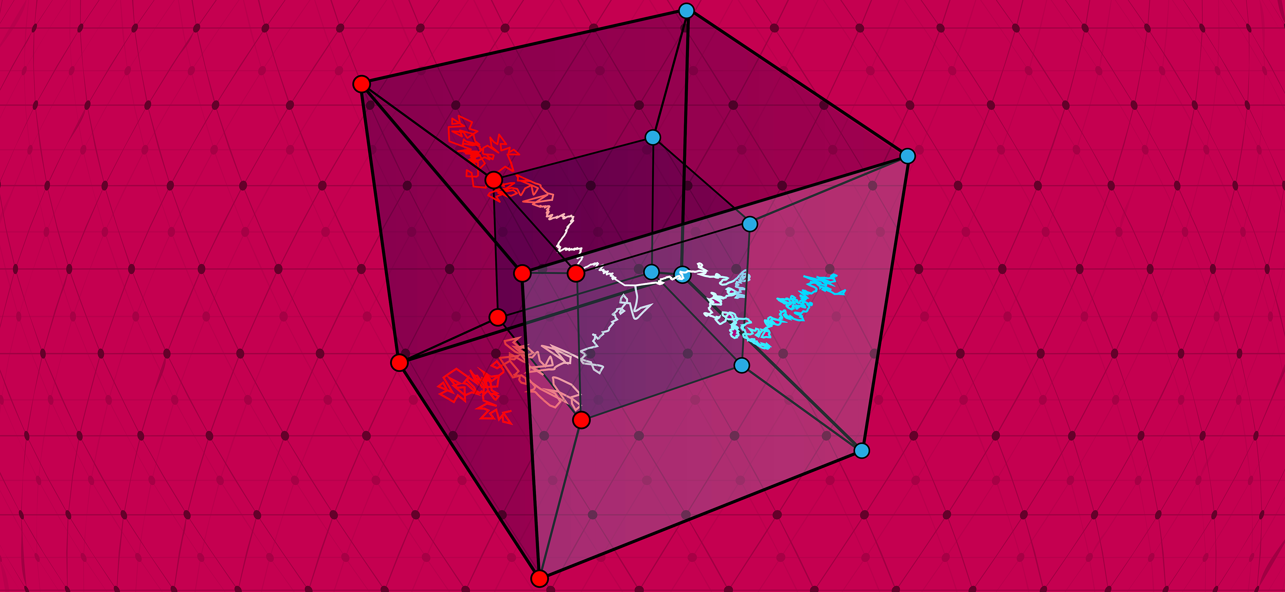
by Jordan Ellenberg (science communicator in residence, Summer 2023)
Some of the richest and most lasting mathematical ideas come about when two distinct fields come together and pay close attention to their intersections. That was the goal of the workshop on Structural Results held at the Simons Institute in July 2023, in which extremal combinatorists and theoretical computer scientists specializing in complexity convened to talk about the overlap between their two fields.
One highlight was Cosmin Pohoata’s talk about his recent breakthrough with Alex Cohen and Dmitrii Zakharov (both still graduate students!) on the Heilbronn triangle problem. It seems like a simple one: If you put n points in a unit square, what is the triangle of smallest area formed by any three of the points? The answer, of course, depends on the location of the points. The question Hans Heilbronn asked in the 1940s was: How large can the smallest triangle be? In other words, how can we arrange the n points so that no three of them form a small triangle? Your first thought might be to arrange the points so that no two of them came too close to each other. But that’s not good enough — if three points are very close to lying on a straight line, the triangle they form will be long but very skinny, and will still have a small area! Indeed, if you toss n points randomly in the square, the smallest triangle you find will typically have an area around 1/n3, but its diameter will be close to that of the square itself! Long skinny triangles are ubiquitous. Komlós, Pintz, and Szemerédi showed in 1981 that there has to be a triangle whose size is at most n-8/7, and there the problem stood for 40 years, until Pohoata and his collaborators broke the 8/7 barrier and showed that the smallest triangle actually has to be a shade smaller — its area is at most n-8/7 – 1/2000.
What do long skinny triangles have to do with computer science? Nothing, per se. But problems about sets of points in space are surprisingly applicable. Tselil Schramm’s talk, for instance (about her joint work with Liu, Mohanty, and Yang). The notion of an expander graph — a network in which a random walk disperses optimally quickly — is crucial to computer science, allowing advances in pseudorandomness, coding theory, and many other areas. Fascinatingly, for many years the situation was the following: it was known that random graphs were expanding with very high probability, but there was no specific family of graphs that could be proved to be expanding! Nowadays there has been an explosion of explicit expanders. But the situation is different in the newer field of high-dimensional expansion, in which instead of networks (which are composed of vertices, some pairs of which are connected by edges) one has complexes, in which the collections of vertices one keeps track of are not just pairs, but triples (or quadruples, or even larger groupings, but the work presented at the workshop was about triples). What Schramm and her collaborators have done is to show that two-dimensional expanders are plentiful (albeit with vertex degree somewhat higher than what one can do in the one-dimensional case), by showing that random constructions really do enjoy this property; in particular, you can take n points at random on a sphere whose dimension is about log n, and take the “edges” to be triples of points which are all within a small distance of each other. Small triangles again! (But this time, “small” in the sense of “all three vertices being mutually close to each other,” not “having small area.”)
What Pohoata’s and Schramm’s work have in common is the difficulty of going from 2 to 3: problems about pairs of points are well understood, but problems about triangles are drastically harder! (This phenomenon is familiar from dynamics, where the two-body problem is a simple matter of ellipses, while the three-body problem remains frustratingly unsolved and an active topic of research.) But where the two papers part ways is in their relationship with randomness. The point of Schramm’s work is to prove that a random configuration of points achieves maximum performance. In the Heilbronn triangle problem, randomly chosen points definitely do not make the smallest triangle maximally big; to get to the optimum, one will have to choose points very, very carefully, perhaps according to the dictates of some yet-undiscovered structure.
This dichotomy between structure and randomness was an ever-present theme during the workshop. We saw it in Julia Wolf’s talk about her joint work with Caroline Terry, which was about a new regularity result concerning subsets of the space of Boolean vectors (strings of 0’s and 1’s). One information-theoretic way in which such a subset A could be thought of as “simple” would be if membership in A depended only on a few coordinates. More generally, one can call A regular if there is some linear projection p to a much lower-dimensional space of Boolean vectors such that membership of v in A depends only on the image of v under p, which carries much less information. What Wolf and Terry show is that a different computational notion of tameness, called “k-stability,” implies “approximate regularity” — that there is some projection p such that the value of p(v) determines membership of v in A with high probability. Now we are getting still closer to questions of computational complexity! And the relation was made even more apparent in Shachar Lovett’s Richard M. Karp Distinguished Lecture on communication complexity. In this talk, the setup is that two players, Xavier and Yelena, are trying to compute the value of a function f(x,y) which takes values in {1,-1}. The function is known to both players, but the problem is that Xavier knows only the value of x and Yelena knows only the value of y. Of course they could share their private values and compute f; but the game here is to compute f(x,y) using as few bits of communication between Xavier and Yelena as possible. This complexity problem is visibly of the same flavor as the regularity question contemplated by Terry and Wolf; and here, too, the exciting work arises when we try to compare this notion of complexity with other notions of a more linear-algebraic flavor.
One of the high points of the week was the open-problem session held on the second afternoon of the workshop. In this informal setting, the pure mathematicians and computer scientists jumped to the board, interrogated each other, and laid out a whole spray of conundrums, some stemming directly from the talks we’d heard or were going to here, others from farther afield. The structure, shall we say, allowed for a certain amount of randomness.

by Venkatesan Guruswami (Simons Institute)
Summer is typically a quiet time on university campuses, but not at the Simons Institute, where two programs — one on Analysis and TCS, and another on Quantum Computing — are buzzing along. One might recall that one of the inaugural programs hosted by the Simons Institute, back in Fall 2013, was Real Analysis in Computer Science. In the decade since, the field has cultivated influential new themes such as global hypercontractivity and spectral independence, incorporated methods based on high-dimensional expanders and stochastic calculus, and also enabled striking applications in hardness of approximation, Markov chain analysis, and coding theory. All this progress makes this an excellent time to reconvene a program on this topic. The Quantum Computing program has a special focus on the power of noisy intermediate-scale quantum (NISQ) devices, a subject of great current practical interest aimed at demonstrating quantum advantage with noisy devices (pre-quantum error correction), with unique challenges for and great synergy with theory.
These programs come on the heels of a very busy spring semester that hosted a program on Meta-Complexity, which I wrote about earlier, and an extended reunion on the theory and practice of Satisfiability. The participants in the latter program were exposed to both the theoretical and the practical aspects of SAT solving in parallel, and especially for junior researchers, getting such a perspective early in their careers provides an unparalleled platform from which to embark on interdisciplinary and high-impact research.
Generating primes, almost deterministically
One of the papers to come out of the Meta-Complexity program, co-authored by a team of five full-time participants in the program (Chen, Lu, Oliveira, Ren, and Santhanam), gives a randomized algorithm that on infinitely many inputs n, runs in poly(n) time and with high probability generates a canonical n-bit prime. A randomized polynomial-time algorithm to generate some n-bit prime is easy, as one can just sample O(n) random n-bit numbers, test them for primality, and output a prime among them. But such an algorithm can output different primes on different runs. A deterministic algorithm outputting a single prime always would be desirable, but such an algorithm remains elusive. A pseudodeterministic algorithm is an intriguing middle ground and is a randomized algorithm that on any input outputs a unique answer with high probability. Motivated by the question of generating canonical primes, the concept of pseudodeterministic algorithms was introduced by Gat and Goldwasser in 2011 and has since received much attention. But a pseudodeterministic polynomial-time algorithm for prime generation remained open, and the present work solves it modulo the caveat of only working infinitely often. Actually, the result has nothing to do with generating primes per se, and works for any property of numbers that occurs sufficiently often and that can be checked in polynomial time (both of which hold for primality).
A few years ago, a subset of the present authors gave a subexponential (i.e., exp(n0.01)) pseudodeterministic algorithm for generating primes (again only for infinitely many lengths). This was based on a win-win argument that converts a conditional hardness-randomness trade-off (a specific uniform version due to Trevisan and Vadhan) into an unconditional pseudodeterministic algorithm. Namely, if a certain PSPACE-complete language L that they construct is not in BPP, then one can build a pseudorandom set of subexponential size that fools polynomial-time randomized algorithms (infinitely often). So in this case, one can derandomize the trivial randomized algorithm to generate primes and get a deterministic subexponential-time algorithm. On the other hand, if L is in BPP, then the polynomial-space algorithm that searches over all n-bit numbers to find the lexicographically smallest prime yields a polynomial-time pseudodeterministic algorithm.
Continue readingby Issa Kohler-Hausmann (Senior Law and Society Fellow, Spring 2022, Simons Institute)1
This work was made possible by the Simons Institute’s Causality program in the spring of 2022, where I was the Law and Society fellow and had the opportunity to learn and discuss with a collection of brilliant scholars thinking about and working on causality and causal modeling. Special gratitude goes to Robin Dembroff, Maegan Fairchild, and Shamik Dasgupta, who participated in the April 2022 Theoretically Speaking event “Noncausal Dependence and Why It Matters for Causal Reasoning.”
Introduction
The term “mechanism” or “causal mechanism” is used in two possibly conflicting ways in causal inference literature. Sometimes “causal mechanism” is used to refer to the chain of causal relations that is unleashed between some stipulated triggering event (let’s call it X) and some outcome of interest (let’s call it Y). When people use the term in this sense, they mean “a causal process through which the effect of a treatment on an outcome comes about.”2 One could think of this use of the term as slowing down a movie about the causal process between the moment when X is unleashed and when Y obtains so that we can see more distinct frames capturing ever-finer-grained descriptions of prior events triggering subsequent events as they unfold over time. This is the in-between sense of “mechanism,” or, as Craver says, “causal betweenness.”3 An expansive methodological literature engages causal mechanisms in the in-between sense under the banner of mediation or indirect effects.4 When used in this way, a causal mechanism M lies in the middle of a causal pathway between X and Y: X→M→Y.
But there is a different sense of “mechanism” that refers to whatever it is about the triggering variable (let’s call it X again) that endows it with the causal powers it has. When people use the term in this inside sense, they mean to pick out the constituents of X, the parts and relations that compose it, or the grounds by virtue of which it obtains. Instead of slowing down the movie of a causal process unfolding over time, this use of “mechanism” calls for zooming into X at a particular slice in time.5
Causal models encode mechanisms in the inside sense insofar as denoting a variable (e.g., X) in the model entails denoting the stuff that builds the innards of X in the model.6 Designating variables expresses how the modeler has chosen to carve up states or events in the world. It entails expressing the boundaries of the relata (represented by variables) in the model, as variables marked out as, for example, X and M are taken to be distinct.7 But variable definition often leaves the innards of each relata designated by a variable name — what’s inside of X and M — opaque. And because most causal models we work with are not expressed in terms of fundamental entities (whatever those are — quarks and leptons, or something), variables are built out of or constituted by other things and connections between those things. The variables take the various states designated in the model because certain facts obtain. Inside causal mechanisms are the intravariable relata and relations that compose the variables and give them their distinctive causal powers.
Questions about mechanisms could be posed in one or the other sense of the term. For example, imagine you have a pile of pills and know with absolute certainty that each pill contains the identical chemical substance and dosage. Now imagine you conduct a randomized controlled trial with these pills to see whether ingesting these pills reduces reported headaches, and you document some average causal effect. Upon completion of the study, you might say: “We still do not know the causal mechanisms involved here.” There are simply two meanings to that query.
One meaning is that you do not know what physical processes in the body ingestion of the pill triggered — what physiological pathways ingestion of the substance brought about and unfolded over time such that headache pain was reduced. This version of the query asks about causal mechanisms in the in-between sense. Alternatively, you could mean that you do not know what was in the pill! That is, you have no idea what stuff did the triggering — you do not know the chemical compound that constituted the little pills you gave to your treated subjects.8 This version of the query asks about causal mechanisms in the inside sense, asking what facts obtained such that the thing designated as the cause occurred.
Sometimes people blur these two uses together.9 However, it is important to maintain this conceptual distinction because the relationship between mechanisms in the inside and in-between senses sets some limits on variable definition within a causal model. Specifically, if you posit some mechanism in the in-between sense in a causal model, then the state or event picked out by that mediator cannot be inside another variable.
Continue reading
by Jessica Hullman (Senior Law and Society Fellow (Fall 2022), Simons Institute)
Theories of sequential decision-making have been around for decades but continue to flourish. The Simons Institute’s Fall 2022 program on Data-Driven Decision Processes provided an excellent overview of recent results in online learning and sequential decision-making. Visiting the Simons Institute as a researcher whose background is in interactive data visualization, I spent some time thinking about how learning theory might advance more applied research related to human-data interaction.
First, it’s worth noting that theories of inference and decision-making remain relatively unintegrated in fields that research data interfaces, including human-computer interaction and visualization. While we might sometimes visualize data simply to generate a historical record, such as to compare points scored across NBA players, most of the time visualization is used to support inference tasks like extrapolating beyond the particular sample to the larger population. Yet beyond a smattering of experimental papers that make use of decision theory, only a handful of works have advocated for theorizing the function of visualizations in the context of frameworks that could provide prescriptive guidance (for example, within the traditions of model checking,1 Bayesian cognition,2 and hypothesis testing3).
A natural question is why. I suspect it may have something to do with the status of visualization as a general-purpose tool that can be put to work to summarize data, persuade viewers to draw certain conclusions from data, or support inferential and decision tasks, sometimes simultaneously. More formal theory requires pinning down the problem more precisely, which might seem reductive. Visualization has also long been associated with the tradition of exploratory data analysis in statistics, in which John Tukey pioneered exposure of the unexpected through graphical displays as an overlooked part of statistical practice.4 Maybe the understanding that visualization is valuable for producing unpredictable insights keeps researchers away from attempting to theorize.
The power of visualization is often touted as providing an external representation that enables the amplification of cognition by allowing natural perceptual processes to aid in identifying patterns in data and freeing up valuable working memory. A key part of this is that a good visualization enables its human user to bring their prior domain knowledge to bear. Similar to how some statistical modelers shy away from the idea of formalizing prior knowledge in applied Bayesian statistics, the role of prior knowledge in visualization-aided analysis may contribute to a seeming bias in the literature toward leaving the human part of the equation untheorized. Instead, we’re left to trust that in supporting exploratory analysis in its various forms, visualization interactions don’t need modeling because the analyst will “know when they see it” and also know what to do about it, whether that means transforming data, collecting more data, making a decision, etc.
All this means that there are many opportunities where statistical theory, data economics, and online learning theory could be helpful for providing a more rigorous theoretical framework in which to answer questions that get at the heart of what visualization is about.
Continue reading