
by Venkatesan Guruswami (Simons Institute)
This semester at the Simons Institute, the Meta-Complexity program is buzzing along with intense activity in the form of multiple reading groups and a weekly seminar, on top of the usual three workshops and boot camp. A large number of complexity theorists have converged at the Institute, including several students, postdocs, and junior researchers. And all this complexity action is intermixed with some good and varied fun in the form of many self-organized social activities.
Theory readers know what complexity is, but what is the “meta” for? An online dictionary definition of “meta” is a term describing something that “consciously references or comments upon its own subject or features” — e.g., “A movie about making a movie is just so meta—especially when the actors criticize the acting.”
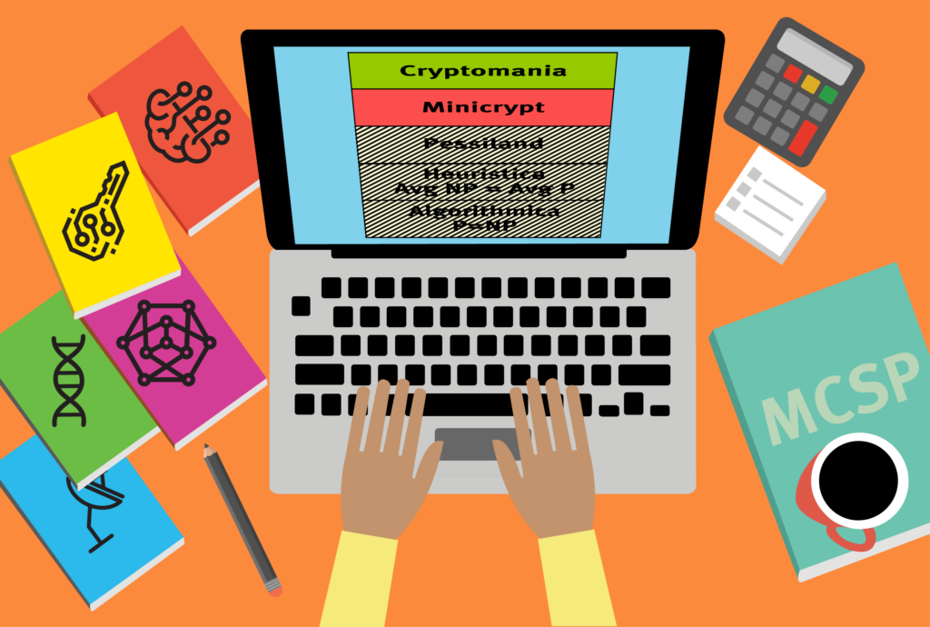
So meta-complexity is the study of complexity of problems that themselves pertain to complexity. A prototypical example is circuit minimization, where the goal is to find the smallest circuit for a given specification. This is modeled as the minimum circuit size problem (MCSP), which is one of the lead actors in meta-complexity: Given the truth table of an n-bit Boolean function f, and a size parameter s, does f have a Boolean circuit of size at most s? (Note that the input size is 2n.)
The MCSP problem was explicitly defined in 2000 by Kabanets and Cai, inspired by Razborov and Rudich’s seminal work on natural proofs from 1994. (Upon some reflection, one can realize that a natural property against some class of circuits is really an average-case, one-sided error algorithm for MCSP on circuits of that class.) Being a “natural” problem, MCSP was in fact considered implicitly even earlier, including in early works on complexity in the former Soviet Union. Yablonski claimed in 1959 that MCSP is not in P (to use modern terminology — the class P wasn’t even defined then). MCSP is easily seen to be in NP — indeed, one can guess a circuit and then check if it computes the function correctly on all inputs — so we of course can’t yet prove that it lies outside P.
Leading up to his seminal work on NP-completeness, Levin was in fact trying to show NP-hardness of MCSP, but didn’t succeed. One of the six problems that Levin showed NP-hardness of was DNF-MCSP, where one tries to find a DNF formula of minimum size to compute a given truth table. (Technically, Levin proved only NP-hardness of the partial-function version of the question, where we don’t care about the function value on some inputs.) In fact, this was Problem 2 on Levin’s list, between Problem 1, which was set cover, and Problem 3, which was Boolean formula satisfiability.
The complexity of MCSP remains open — we do not know if it is in P or NP-complete. Resolving this is a natural challenge, but on the surface it might seem like a rather specific curiosity. One reason to care about MCSP is that any NP-hardness proof faces some fundamental challenges — in particular, the function produced on No instances must have large circuits, giving an explicit function in EXP that has large circuits, which seems beyond the reach of current techniques. One might try to circumvent this via randomized or exponential-time reductions, and this has indeed fueled some very interesting recent results, as well as intriguing connections to learning theory, average-case complexity, cryptography, and pseudorandomness.
An “extraneous” reason to care about MCSP and meta-complexity is that the underlying techniques have led to some of the best insights on certain foundational questions that have nothing to do with meta-complexity per se. Meta-complexity has been energized by some significant recent progress on both of these (internal and extraneous) fronts. These advances and momentum are fueling a lot of activity and optimism in the Simons Institute program this semester.
CONTINUE READING
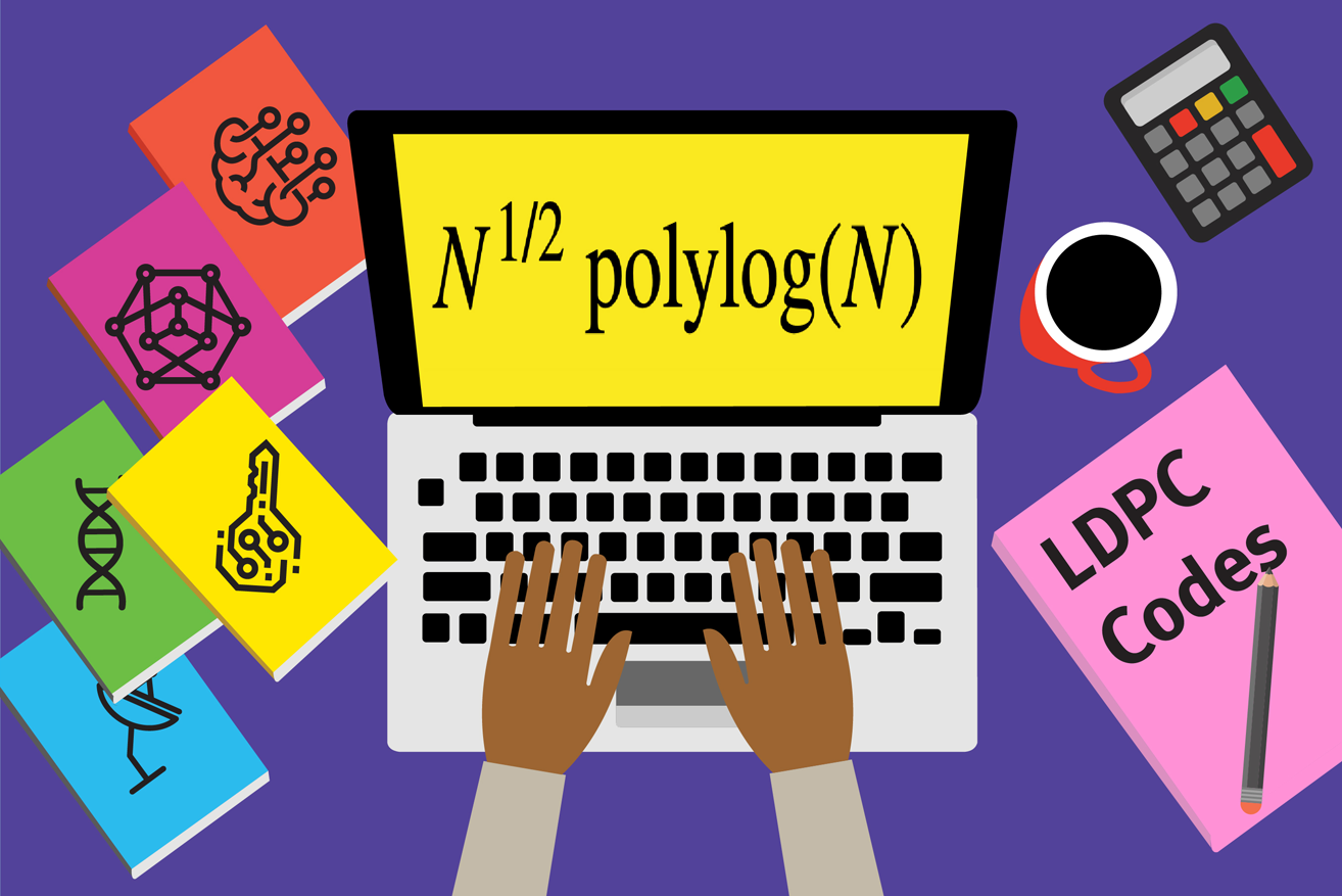 It has been only a few months since the last time this column appeared. Yet there is so much to write about that it feels like a year has passed. For one area in particular, a decade’s worth of developments seems to have emerged in a few months’ time. I am talking of course about the phenomenal developments on error-correcting codes that we witnessed in the past few months.
 Being in one of the talks in the Simons Institute auditorium, witnessing live and lively interaction with the speaker, feels like the closest thing to normal since the start of the pandemic. There is a sense of tangible joy among the participants just to be sharing the same physical space, let alone the fantastic environs of the Institute. The renewed energy is all there to witness in the programs this semester on
  Another semester of remote activities at the Simons Institute draws to a close. In our second semester of remote operations, many of the quirks of running programs online had been ironed out. But pesky challenges such as participants being in different time zones remained. To cope with these, the programs spread their workshop activities throughout the semester. Not only did this help with the time zones, but it helped keep up the intensity all through the semester.
 Blockchains and decentralized ledgers are creating a new reality for modern society. A major scientific impact of this new reality is that it creates an interdisciplinary arena where traditionally independent research areas, such as cryptography and game theory/economics, need to work together to address the relevant questions. The Simons Institute’s Fall 2019 program on