Lattice Blog Reduction – Part III: Self-Dual BKZ

This is the third and last entry in a series of posts about lattice block reduction. See here and here for the first and second parts, resp. In this post I will assume you have read the other parts.

In the first two parts we looked at BKZ and Slide reduction, the former being the oldest and most useful in practice, while the latter achieves the best provable bounds and has the cleaner analysis. While BKZ is a natural generalization of LLL, we have seen that the analysis of LLL does not generalize well to BKZ. One can view Slide reduction as a different generalization of LLL with the goal of also naturally generalizing its analysis. As we mentioned in the first part, there is another analysis technique based on dynamical systems, introduced in [HPS11]. Unfortunately, as applied to BKZ, there are some cumbersome technicalities and the resulting bounds on the output quality are not as tight as we would like them to be (i.e. as for Slide reduction). One can view the algorithm we are considering today – SDBKZ [MW16] – as a generalization of LLL that lends itself much easier to this dynamical systems analysis: it is simpler, cleaner and yields better results. Since part of the goal of today’s post is to demonstrate this very useful analysis technique, SDBKZ is a natural candidate.

SDBKZ

Recall the two tools we’ve been relying on in the first two algorithms, SVP and DSVP reduction of projected subblocks:

Effect of a call to the DSVP oracle. GSO log norms of the input in black, of the output in blue. Note that the sum of the GSO log norms is a constant, so increasing the length of the last vector, decreases the (average of the) remaining vectors.

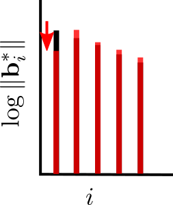
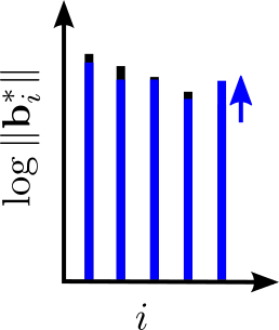
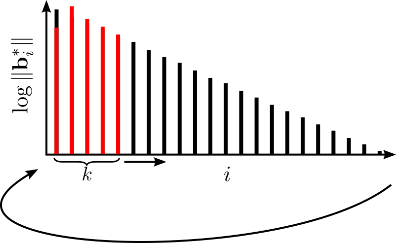
We will use both of them again today. Like BKZ, a tour of SDBKZ starts by calling the SVP oracle on successive blocks of our basis. However, when we reach the end of the basis, we will not decrease the size of the window, since this is actually quite inconvenient for the analysis. Instead, we will keep the size of the window constant but switch to DSVP reduction, i.e. at the end of the BKZ tour we DSVP reduce the last block. This will locally maximize the last GSO vector in the basis, just as the first SVP call locally minimized the first vector of the basis. Then we will move the window successively backwards, mirroring a BKZ tour, but using DSVP reduction, until we reach the beginning of the basis again. At this point, we switch back to SVP reduction and move the window forward, etc. So SDBKZ runs in forward and backward tours.

SDBKZ in one picture: apply the SVP oracle to the projected blocks from start to finish and when you reach the end, apply the DSVP oracle to from finish to start. Repeat.

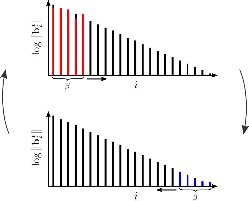
A nice observation here is that the backward tour can be viewed equivalently as: 1) compute the reversed dual basis (i.e. the dual basis with reversed columns), 2) run a forward tour, 3) compute the primal basis again. The first of these two steps is self-inverse: computing the reversed dual basis of the reversed dual basis yields the original primal basis. This means step 3) is actually the same as step 1). So in effect, one can view SDBKZ as simply repeating the following two steps: 1) run a forward tour, 2) compute the reversed dual basis. So it doesn’t matter if we use the primal or the dual basis as input, the operations of the algorithm are the same. This is why it is called Self-Dual BKZ.

There is one caveat with this algorithm: it is not clear, when one should terminate. In BKZ and Slide reduction one can formulate clear criteria, when the algorithm makes no more progress anymore. In SDBKZ this is not the case, but the analysis will show that we can bound the number of required tours ahead of time.

The Analysis

We will start by analyzing the effect of a forward tour. Let \({\mathbf{B}}\) be our input basis. The first call to the SVP oracle in a forward tour replaces \({\mathbf{b}}_1\) with the shortest vector in \({\mathbf{B}}_{[1,k]}\). This means that the new basis \({\mathbf{B}}’\) satifies \(\| {\mathbf{b}}_1′ \| \leq \sqrt{\gamma_k} (\prod_{i=1}^k \|{\mathbf{b}}_i^* \|)^{1/k}\) by Minkowski’s bound. Equivalently, this can be written as \[\log \| {\mathbf{b}}_1′ \| \leq \log \sqrt{\gamma_k} + \frac1k (\sum_{i=1}^k \log \|{\mathbf{b}}_i^* \|).\] So if we consider the \(\log \|{\mathbf{b}}_i^*\|\) as variables, it seems like linear algebra could be useful here. So far, so good. The second step is more tricky though. We know that the next basis \({\mathbf{B}}”\), i.e. after the call to the SVP oracle on \({\mathbf{B}}’_{[2,k+1]}\), satisfies \({\mathbf{b}}_1” = {\mathbf{b}}_1’\) and \(\| ({\mathbf{b}}_2”)^* \| \leq \sqrt{\gamma_k} (\prod_{i=2}^{k+1} \|({\mathbf{b}}’_i)^* \|)^{1/k}\). Unfortunately, we have no control over \(\|({\mathbf{b}}’_i)^* \|\) for \(i \in {2,\dots,k} \), since we do not know how the SVP oracle in the first call changed these vector. However, we do know that the lattice \({\mathbf{B}}_{[1,k+1]}\) did not change in that call. So we can write \[\prod_{i=2}^{k+1} \|({\mathbf{b}}’_i)^* \| = \frac{\prod_{i=1}^{k+1} \|{\mathbf{b}}_i^* \|}{\| {\mathbf{b}}’_1 \|}\] and thus we obtain \[\log \| ({\mathbf{b}}_2′)^* \| \leq \log \sqrt{\gamma_k} + \frac1k (\sum_{i=1}^{k+1} \log \|{\mathbf{b}}_i^* \| – \log \|{\mathbf{b}}’_1 \|).\] Again, this looks fairly “linear algebraicy”, so it could be useful. But there is another issue now: in order to get an inequality purely in the input basis \({\mathbf{B}}\), we would like to use our inequality for \(\log \|{\mathbf{b}}_1′ \|\) in the one for \(\log \| ({\mathbf{b}}_2′)^* \|\). But the coefficient of \(\log \|{\mathbf{b}}_1′ \|\) is negative, so we would need a lower bound for \(\log \|{\mathbf{b}}_1′ \|\). Furthermore, we would like to use upper bounds for our variables later, since the analysis of a tour will result in upper bounds and we would like to apply it iteratively. For this, negative coefficients are a problem. So, we need one more modification: we will use a change of variable to fix this. Instead of considering the variables \(\log \| {\mathbf{b}}_i^* \|\), we let the input variables to our forward tour be \(x_i = \sum_{j < k+i} \log \|{\mathbf{b}}^*_i \|\) and the output variables \(y_i = \sum_{j \leq i} \log \|({\mathbf{b}}’_i)^* \|\) for \(i \in [1,\dots,n-k]\). Clearly, we can now write our upper bound on \(\log \|({\mathbf{b}}’_1)^*\|\) as \[y_1 \leq \log \sqrt{\gamma_k} + \frac{x_1}{k}.\] More generally, we have \[\|({\mathbf{b}}’_i)^* \| \leq \sqrt{\gamma_k} \left(\frac{\prod_{j=1}^{i+k-1} \|{\mathbf{b}}_j^* \|}{\prod_{j=1}^{i-1} \|({\mathbf{b}}’_j)^* \|} \right)^{\frac1k}\] which means for our variables \(x_i\) and \(y_i\) that \[y_i = y_{i-1} + \log \| ({\mathbf{b}}’_i)^* \| \leq y_{i-1} + \log \sqrt{\gamma_k} + \frac{x_i – y_{i-1}}{k} = (1-\frac1k) y_{i-1} + \frac1k x_i + \log \sqrt{\gamma_k}.\]

Note that we can write each \(y_i\) in terms of \(x_i\) and the previous \(y_i\) with only positive coefficients. So now we can apply induction to write each \(y_i\) only in terms of the \(x_i\)’s, which shows that \[y_i = \frac1k \sum_{j=1}^i \omega^{i-j} x_j + (1-\omega)^i k \alpha\] where we simplified notation a little by defining \(\alpha = \log \sqrt{\gamma_k}\) and \(\omega = 1-\frac1k\). By collecting the \(x_i\)’s and \(y_i\)’s in a vector each, we have the vectorial inequality \[{\mathbf{y}} \leq {\mathbf{A}} {\mathbf{x}} + {\mathbf{b}}\] where \[{\mathbf{b}} = \alpha k \left[ \begin{array}{c} 1 – \omega \\ \vdots \\ 1 – \omega^{n-k} \end{array}\right] \qquad\qquad {\mathbf{A}} = \frac1k \left[ \begin{array}{cccc} 1 & & & \\ \omega & 1 & & \\ \vdots & \ddots & \ddots & \\ \omega^{n-k-1} & \cdots & \omega & 1 \end{array} \right].\]

Now recall that after a forward tour, SDBKZ computes the reversed dual basis. Given the close relationship between the primal and the dual basis and their GSO, one can show that simply reversing the vector \({\mathbf{y}}\) will yield the right variables \({\mathbf{x}}’_i\) to start the next “forward tour” (which is actually a backward tour, but on the dual). I.e. after reversing \({\mathbf{y}}\), the variables represent the logarithm of the corresponding subdeterminants of the dual basis. (For this we assume for convenience and w.l.o.g. that the lattice has determinant 1; otherwise, there would be a scaling factor involved in this transformation.)

In summary, the effect on the vector \({\mathbf{x}}\) of executing once the two steps, 1) forward tour and 2) computing the reversed dual basis, can be described as \[{\mathbf{x}}’ \leq {\mathbf{R}} {\mathbf{A}} {\mathbf{x}} + {\mathbf{R}} {\mathbf{b}}\] where \({\mathbf{R}}\) is the reversed identity matrix (i.e. the identity matrix with reversed columns). Iterating the two steps simply means we will be iterating the vectorial inequality above. So analyzing the affine dynamical system \[{\mathbf{x}} \mapsto {\mathbf{R}} {\mathbf{A}} {\mathbf{x}} + {\mathbf{R}} {\mathbf{b}}\] will allow us to deduce information about the basis after a certain number of iterations.

Small Digression: Affine Dynamical Systems

Consider some dynamical system \({\mathbf{x}} \mapsto {\mathbf{A}} {\mathbf{x}} + {\mathbf{b}} \) and assume it has exactly one fixed point, i.e. \({\mathbf{x}}^*\) such that \({\mathbf{A}} {\mathbf{x}}^* + {\mathbf{b}} = {\mathbf{x}}^* \). We can write any input \({\mathbf{x}}’\) as \({\mathbf{x}}’ = {\mathbf{x}}^* + {\mathbf{e}}\) for some “error vector” \({\mathbf{e}}\). When applying the system to it, we get \({\mathbf{x}}’ \mapsto {\mathbf{A}} {\mathbf{x}}’ + {\mathbf{b}} = {\mathbf{x}}^* + {\mathbf{A}} {\mathbf{e}}\). So the error vector \({\mathbf{e}}\) is mapped to \({\mathbf{A}} {\mathbf{e}}\). Applying this \(t\) times maps \({\mathbf{e}}\) to \({\mathbf{A}}^t {\mathbf{e}}\), which means after \(t\) iterations the error vector has norm \(\|{\mathbf{A}}^t {\mathbf{e}} \|_{p} \leq \|{\mathbf{A}}^t \|_{p} \| {\mathbf{e}} \|_{p} \) (where \(\| \cdot \|_{p}\) is the matrix norm induced by the vector \(p\)-norm). If we can show that \(\|{\mathbf{A}} \|_p \leq 1 – \epsilon\), then \(\|{\mathbf{A}}^t \|_p \leq \|A \|^t \leq (1-\epsilon)^t \leq e^{-\epsilon t}\), so the error vector will decay exponentially in \(t\) with base \(e^{-\epsilon}\) and the algorithm converges to the fixed point \({\mathbf{x}}^*\).

Back to our concrete system above. As we just saw, we can analyze its output quality by computing its fixed point and its running time by computing \(\|{\mathbf{R}} {\mathbf{A}} \|_p\) for some induced matrix \(p\)-norm. Since this has been a lenghty post already, I hope you’ll trust me that our system above has a fixed point \({\mathbf{x}}^*\), which can be written out explicitely in closed form. As a teaser, its first coordinate is \[x^*_1 = \frac{(n-k)k}{k-1} \alpha.\] This means that if the algorithm converges, it will converge to a basis such that \(\sum_{j \leq k}\log \| {\mathbf{b}}_j^*\| \leq \frac{(n-k)k}{k-1} \log \sqrt{\gamma_k}\). Applying Minkowski’s Theorem to the first block \({\mathbf{B}}_{[1,k]}\) now shows that the shortest vector in this block satisfies \(\lambda_1({\mathbf{B}}_{[1,k]}) \leq \sqrt{\gamma_k}^{\frac{n-1}{k-1}}\). Note that the next forward tour will find a vector of such length. Recall that we assumed that our lattice has determinant 1, so this is exactly the Hermite factor achieved by Slide reduction, but for arbitrary block size (we do not need to assume that \(k\) divides \(n\)) and better than what we can achieve for BKZ (even using the same technique). Moreover, the fixed point actually gives us more information: the other coordinates (that I have ommited here) allow us control over all but \(k\) GSO vectors and by terminating the algorithm at different positions, it allows us to choose which vectors we want control over.

It remains to show that the algorithm actually converges and figure out how fast. It is fairly straight-forward to show that \[\|{\mathbf{R}} {\mathbf{A}}\|_{\infty} = \|{\mathbf{A}}\|_{\infty} = 1 – \omega^{n-k} \approx e^{-\frac{n-k}{k}}.\] (Consider the last row of \({\mathbf{A}}\).) This is always smaller than 1, so the algorithm does indeed converge. For \(k = \Omega(n)\) this is bounded far enough from 1 such that the system will converge to the fixed point up to an arbitrary constant in a number of SVP calls that is polynomial in \(n\). Using another change of variable [N16] or considering the relative error instead of the absolute error [MW15], one can show that this also holds for smaller \(k\).

As mentioned before, this type of analysis was introduced in [HPS11] and has inspired new ideas even in the heuristic analysis of BKZ. In particular, one can predict the behavior of BKZ by simply running such a dynamical system on typical inputs (and making some heuristic assumptions). This idea has been and is being used extensively in cryptanalysis and in optimizing parameters of state-of-the-art algorithms.

Finally, a few last words on SDBKZ: we have seen that it achieves a good Hermite factor, but what can we say about the approximation factor? I actually do not know if the algorithm achieves a good approximation factor and also do not see a good way to analyze it. However, there is a reduction [L86] from achieving approximation factor \(\alpha\) to achieving Hermite factor \(\sqrt{\alpha}\). So SDBKZ can be used to achieve approximation factor \(\gamma_k^{\frac{n-1}{k-1}}\). This is a little unsatisfactory in two ways: 1) the reduction results in a different algorithm, and 2) the bound is a little worse than the factor achieved by slide reduction, which is \(\gamma_k^{\frac{n-k}{k-1}}\). On a positive note, a recent work [ALNS20] has shown that, due to the strong bound on the Hermite factor, SDBKZ can be used to generalize Slide reduction to arbitrary block size \(k\) in a way to achieve the approximation factor \(\gamma_k^{\frac{n-k}{k-1}}\). Another recent work [ABFKSW20] exploited the fact that SDBKZ allows to heuristically predict large parts of the basis to achieve better bounds on the running time of the SVP oracle.

  • Lovász. An Algorithmic Theory of Numbers, Graphs and Convexity. 1986

  • Hanrot, Pujol, Stehlé. Analyzing blockwise lattice algorithms using dynamical systems. CRYPTO 2011

  • Micciancio, Walter. Practical, predictable lattice basis reduction – Full Version. http://eprint.iacr.org/2015/1123

  • Micciancio, Walter. Practical, predictable lattice basis reduction. EUROCRYPT 2016

  • Neumaier. Bounding basis reduction properties. Designs, Codes and Cryptography 2016

  • Aggarwal, Li, Nguyen, Stephens-Davidowitz. Slide Reduction, Revisited—Filling the Gaps in SVP Approximation. CRYPTO 2020

  • Albrecht, Bai, Fouque, Kirchner, Stehlé, Wen. Faster Enumeration-based Lattice Reduction: Root Hermite Factor \(k^{(1/(2k))}\) in Time \(k^{(k/8 + o(k))}\). CRYPTO 2020

Lattice Blog Reduction – Part I: BKZ

This is the first entry in a (planned) series of at least three, potentially four or five, posts about lattice block reduction. The purpose of this series is to give a high level introduction to the most popular algorithms and their analysis, with pointers to the literature for more details. The idea is to start with the obvious – the classic BKZ algorithm. In the next two posts we will look at two lesser known algorithm, which allow to highlight useful tools in lattice reduction. These three posts will focus on provable results. I have not decided how to proceed from there, but I could see the series being extended to topics involving heuristic analyses, practical considerations, and/or a survey of more exotic algorithms that have been considered in the literature.

Target Audience

I will assume that readers of this series are already familiar with basic concepts of lattices, e.g. bases, determinants, successive minima, Minkowski’s bound, Gram-Schmidt orthogonalization, dual lattices and dual bases, etc. If any of these concepts seem new to you, there are great resources to familiarize yourself with them first (see e.g. lecture notes by Daniele, Oded, Daniel/Léo). It will probably help if you are familiar with the LLL algorithm (also covered in aforementioned notes), but I’ll try to phrase everything so it is understandable even if if you aren’t.

Ok, so let’s get started. Before we look at BKZ in particular, first some comments about lattice block reduction in general.

The Basics

The Goal

Why would anyone use block reduction? There are (at least) two reasons.

1) Block reduction allows you to find short vectors in a lattice. Recall that finding the shortest vector in a lattice (i.e. solving SVP) is really hard (as far as we know, this takes at least \(2^{\Omega(n)}\) time or even \(n^{\Omega(n)}\) if you are not willing to also spend exponential amounts of memory). On the other hand, finding somewhat short vectors that are longer than the shortest vector by “only” an exponential factor is really easy (see LLL). So what do you do if you need something that is shorter than what LLL gives you, but you don’t have enough time to actually find the shortest vector? (This situation arises practically every time you use lattice reduction for cryptanalysis.) You can try to find something in between and hope that it doesn’t take as long. This is where lattice reduction comes in: it gives you a smooth trade-off between the two settings. It is worth mentioning that when it comes to approximation algorithms, block reduction is essentially the only game in town, i.e. there are, as far as I know, no non-trivial approximation algorithms that cannot be viewed as block reduction. (In fact, this is related to an open problem that Noah stated during the program: to come up with a non-trivial approximation algorithm that does not rely on a subroutine to find the shortest lattice vector in smaller dimensions.) The only exception to this are quantum algorithms that are able to find subexponential approximations in polynomial time in lattices with certain (cryptographically highly relevant) structure (see [CDPR16] and follow up work).

2) Block reduction actually gives you more than just short vectors. It gives you guarantees on the “quality” of the basis. What do we mean by the quality of the basis? Consider the Gram-Schmidt vectors \({\mathbf{b}}_i^*\) (GSO vectors) associated to a lattice basis \({\mathbf{B}}\). What we want is that the length of these Gram-Schmidt vectors (the GSO norms) does not drop off too quickly. The reason why this is a useful measure of quality for lattice bases is that it gives a sense of how orthogonal the basis vectors are: conditioned on being bases of the same lattice, the less accentuated the drop off in the GSO vectors, the more orthogonal the basis, and the more useful this basis is to solve several problems in a lattice. In fact, recall that the product of the GSO norms is equal to the determinant of the lattice and thus remains constant. Accordingly, if the GSO norms do not drop off too quickly, the first vector can be shown to be relatively short. So by analyzing the quality of the basis that block reduction achieves, a guarantee on the length of the first vector comes for free (see goal 1)). If you are familiar with the analysis of LLL, this should not come as a surprise to you.

Tools

In order to ensure that the GSO norms do not drop off to quickly, it seems useful to be able to reduce them locally. To this end, we will work with projected lattice blocks (this is where the term “block” in block reduction comes from). More formally, given a basis \({\mathbf{B}}\) we will consider the block \({\mathbf{B}}_{[i,j]}\) for \(i < j\) as the basis formed by the basis vectors \({\mathbf{b}}_i, {\mathbf{b}}_{i+1}, \dots, {\mathbf{b}}_{j}\) projected orthogonally to the first \(i-1\) basis vectors. So \({\mathbf{B}}_{[i,j]}\) is a basis for the lattice given by the sublattice formed by \({\mathbf{b}}_1, {\mathbf{b}}_{2}, \dots, {\mathbf{b}}_{j}\) projected onto the orthogonal subspace of the vectors \({\mathbf{b}}_1, {\mathbf{b}}_{2}, \dots, {\mathbf{b}}_{i-1}\). Notice that the first vector of \({\mathbf{B}}_{[i,j]}\) is exactly \({\mathbf{b}}^*_i\) – the \(i\)-th GSO vector. Another way to view this is to consider the QR-factorization of \({\mathbf{B}} = {\mathbf{Q}} {\mathbf{R}}\), where \({\mathbf{B}}\) is the matrix whose columns are the basis vectors \({\mathbf{b}}_i\). Since \({\mathbf{Q}}\) is orthonormal, it represents a rotation of the lattice and we can consider the lattice generated by the columns of \({\mathbf{R}}\) instead, which is an upper triangular matrix. For an upper triangular basis, the projection of a basis vector orthogonal to the previous basis vectors simply results in dropping the first entries from the vector. So considering a projected block \({\mathbf{R}}_{i,j}\) is simply to consider the square submatrix of \({\mathbf{R}}\) consisting of the rows and columns with index \(k\) between \(i \leq k \leq j\).

Now we need a tool that allows us to control these GSO vectors, which we view as the first basis vectors in projected sublattices. For this, we will fall back to algorithms that solve SVP. Recall that this is very expensive, so we will not call this on the basis \({\mathbf{B}}\) but rather on the projected blocks \({\mathbf{B}}_{[i,j]}\), where we ensure that the dimension \(k = j-i+1\) of the lattice generated by this projected block is not too large. In fact, the maximum dimension \(k\) that we call the SVP algorithm on will control the time/quality trade-off achieved by our block reduction algorithms and is usually denoted by the block size. So we will assume that we have access to such an SVP algorithm. Actually, we will assume something slightly stronger: we will assume access to a subroutine that takes as input the basis \({\mathbf{B}}\) and indices \(i,j\) and outputs a basis \({\mathbf{C}}\) such that

  • the lattice generated by the basis remains the same

  • the first \(i-1\) and the last vectors starting from \(j+1\) remain unchanged

  • the projected block \({\mathbf{C}}_{[i,j]}\) is SVP reduced, meaning that \({\mathbf{c}}^*_i\) is the shortest vector in the lattice generated by \({\mathbf{C}}_{[i,j]}\). Additionally, if \({\mathbf{B}}_{[i,j]}\) is already SVP reduced, we assume that the basis \({\mathbf{B}}\) is left unchanged.

We will call an algorithm that achieves this an SVP oracle. Such an oracle can be implemented given any algorithm that solves SVP (for arbitrary lattices). The technical detail of filling in the gap is left as homework to the reader.

Effect of a call to the SVP oracle. GSO log norms of the input in black, of the output in red. Note that the sum of the GSO log norms is a constant, so reducing the first vector, increases the (average of the) remaining vectors.

For the analysis we need to know what such an SVP oracle buys us. This is where Minkowski’s theorem comes in: we know that for any \(n\)-dimensional lattice \(\Lambda\) we have \(\lambda_1(\Lambda) \leq \sqrt{\gamma_n} \det(\Lambda)^{1/n}\) (where \(\lambda_1(\Lambda)\) is the length of the shortest vector in \(\Lambda\) and \(\gamma_n = \Theta(n)\) is Hermite’s constant). This tells us that after we’ve applied the SVP oracle to a projected block \({\mathbf{B}}_{[i,i+k-1]}\), we have \[\|{\mathbf{b}}^*_i \| \leq \sqrt{\gamma_{k}} \left(\prod_{j = i}^{i+k-1} \|{\mathbf{b}}_j^* \| \right)^{1/k}.\] Almost all of the analyses of block reduction algorithms, at least in terms of their output quality, rely on this single inequality.

Disclaimer

Before we finally get to talk about BKZ, I want to remark that throughout this series I will punt on a technical (but very important) topic: the number of arithmetic operations (outside of the oracle calls) and the size of the numbers. The number of arithmetic operations is usually not a problem, since it will be dominated by the calls to the SVP oracle. We will only compute projections of sublattices corresponding to projected blocks as described above to pass them to the oracle, which can be done efficiently using the Gram-Schmidt orthogonalization. The size of the numbers is a more delicate issue. We need to ensure that the required precision for these projections does not explode somehow. This is usually addressed by interleaving the calls to the SVP oracle with calls to LLL. If you are familiar with the LLL algorithm, it should be intuitive that this allows to control the size of the number. For a clean example of how this can be handled, we refer to e.g. [GN08a]. So, in summary, we will measure the running time of our algorithms thoughout simply in the number of calls to the SVP oracle.

BKZ

Schnorr [S87] introduced the concept of BKZ reduction in the 80’s as a generalization of LLL. The first version of the BKZ algorithm as we consider it today was proposed by Schnorr and Euchner [SE94] a few years later. With our setup above, the algorithm can be described in a very simple way. Let \({\mathbf{B}}\) be a lattice basis of an \(n\)-dimensional lattice and \(k\) be the block size. Recall that this is a parameter that will determine the time/quality trade-off as we shall see in the analysis. We start by calling the SVP oracle on the first block \({\mathbf{B}}_{[1,k]}\) of size \(k\). Once this block is SVP reduced, we shift our attention to the next block \({\mathbf{B}}_{[2,k+1]}\) and call the oracle on that. Notice that SVP reduction of \({\mathbf{B}}_{[2,k+1]}\) may change the lattice generated by \({\mathbf{B}}_{[1,k]}\) and \({\mathbf{b}}_1\) may not be the shortest vector in the first block anymore, i.e. it can potentially be reduced even further. However, instead of going back and fixing that, we will simply leave this as a problem to “future us”. For now, we continue in this fashion until we reach the end of the basis, i.e. until we called the oracle on \({\mathbf{B}}_{n-k,n}\). Note that so far this can be viewed as considering a constant sized window moving from the start of the basis to the end and reducing the first vector of the projected block in this window as much as possible using the oracle. Once we have reached the end of the basis, we start reducing the window size, i.e. we call the oracle on \({\mathbf{B}}_{n-k+1,n}\), then on \({\mathbf{B}}_{n-k+2,n}\), etc. This whole process is called a BKZ tour.

Now that we have finished a tour, it is time to go back and fix the blocks that are not SVP reduced anymore. We do this simply by running another tour. Again, if the second tour modified the basis, there is no guarantee that all the blocks are SVP redcued. So we simply repeat, and repeat, and … you get the idea. We run as many tours as required until the basis does not change anymore. That’s it. If this looks familiar to you, that’s not a coincidence: if we plug in \(k=2\) as our block size, we obtain (a version of) LLL! So BKZ is a proper generalization of LLL.

BKZ in one picture: apply the SVP oracle to the projected blocks from start to finish and when you reach the end, repeat.

The obvious questions now are: what can we expect from the output? And how long does it take?

The Good

We will now take a closer look at the approximation factor achieved by BKZ. If you want to follow this analysis along, you might want to get out pen and paper. Otherwise, feel free to trust me on the calculations (I wouldn’t!) and/or jump ahead to the end of this section for the result (no spoilers!). Let’s assume for now that the BKZ algorithm terminates. If it does, we know that the projected block \({\mathbf{B}}_{[i, i+k-1]}\) is SVP reduced for every \(i \in [1,\dots,n-k+1]\). This means that we have \[\|{\mathbf{b}}^*_i \|^k \leq \gamma_{k}^{k/2} \prod_{j = i}^{i+k-1} \|{\mathbf{b}}_j^* \|\] for all these \(n-k+1\) values of \(i\). Multiplying all of these inequalities and canceling terms gives the inequality \[\|{\mathbf{b}}^*_1 \|^{k-1}\|{\mathbf{b}}^*_2 \|^{k-2} \dots \|{\mathbf{b}}^*_{k-1} \| \leq \gamma_{k}^{\frac{(n-k+1)k}{2}} \|{\mathbf{b}}_{n-k+2}^* \|^{k-1} \|{\mathbf{b}}_{n-k+3}^* \|^{k-2} \dots \|{\mathbf{b}}_{n}^* \|.\] Now we make two more observations: 1) not only is \({\mathbf{B}}_{[1, k]}\) SVP reduced, but so is \({\mathbf{B}}_{[1, i]}\) for every \(i < k\). (Why? Think about it for 2 seconds!) This means we can multiply the inequalities \[\|{\mathbf{b}}^*_1 \|^i \leq \gamma_{i}^{i/2} \prod_{j = 1}^{i} \|{\mathbf{b}}_j^* \|\] for all \(i \in [2,k-1]\) together with the trivial inequality \(\|{\mathbf{b}}^*_1 \| \leq \|{\mathbf{b}}^*_1 \|\), which gives \[\|{\mathbf{b}}^*_1 \|^{\frac{k(k-1)}{2}} \leq \left(\prod_{i = 2}^{k-1} \gamma_{i}^{i/2} \right) \prod_{i = 1}^{k-1} \|{\mathbf{b}}_i^* \|^{k-1}\] Now we use the fact that \(\gamma_k^k \geq \gamma_i^i\) for all \(i \leq k\) (Why? Homework!) and combine with our long inequality above to get \[\|{\mathbf{b}}^*_1 \|^{\frac{k(k-1)}{2}} \leq \gamma_k^{\frac{k(n-1)}{2}} \|{\mathbf{b}}_{n-k+2}^* \|^{k-1} \|{\mathbf{b}}_{n-k+3}^* \|^{k-2} \dots \|{\mathbf{b}}_{n}^* \|.\] (I’m aware that this is a lengthy calculation for a blog post, but we’re almost there, so bear with me. It’s worth it!)

We now use one final observation, which is a pretty common trick in lattice algorithms: w.l.o.g. assume that for some shortest vector \({\mathbf{v}}\) in our lattice its projection orthogonal to the first \(n-1\) basis vectors is non-zero (if it is zero for all of the shortest vectors, simply drop the last vector from the basis, the result is still BKZ reduced, so use induction). Then we must have that \(\lambda_1 = \| {\mathbf{v}} \| \geq \|{\mathbf{b}}_i^* \|\) for all \(i \in [n-k+2, \dots, n]\), since otherwise the projected block \({\mathbf{B}}_{i,n}\) would not be SVP reduced. This means, we have \(\lambda_1 \geq \max_{i \in [n-k+2, \dots, n]} \|{\mathbf{b}}_i^* \|\). This is the final puzzle piece to get our approximation bound: \[\|{\mathbf{b}}^*_1 \| \leq \gamma_{k}^{\frac{n-1}{k-1}} \lambda_1.\] Note that this analysis (dating back to Schnorr [S94]) is reminiscent of the analysis of LLL and if we plug in \(k=2\), we get exactly what we’d expect from LLL. Though we do note a gap in the other extreme: if we plug in \(k=n\), we know that the approximation factor is \(1\) (we are solving SVP in the entire lattice), but the bound above yields a factor \(\gamma_n = \Theta(n)\).

The Bad

Now that we’ve looked at the output quality of the basis, let’s see what we can say about the running time (recall that our focus is on the number of calls to the SVP oracle). The short answer is: not much and that’s very unfortunate. Ideally, we’d want a bound on the number of SVP calls that is polynomial in \(n\) and \(k\). This would mean that the overall running time for large \(k\) is dominated by the running time of the SVP oracle in dimension \(k\) and the block size would give us exactly the expected trade-off. However, an LLL style analysis has so far only yielded a bound on the number of tours which is \(O(k^n)\) [HPS11, Appendix]. This is quite bad – for large \(k\) the number of calls will be the dominating factor in the running time.

The Ugly

Recall that the analysis of LLL does not only provide a bound on the approximation factor, but also on the Hermite factor, i.e. on the ratio of \(\| {\mathbf{b}}_1\|/\det(\Lambda)^{1/n}\). Since an LLL-style analysis worked out nicely for the approximation factor of BKZ, it stands to reason that a similar analysis should yield a similar bound for BKZ. By extrapolating from LLL, one could expect a bound along the lines of \(\| {\mathbf{b}}_1\|/\det(\Lambda)^{1/n} \leq \gamma_{k}^{n/2k}\) (note the square root improvement w.r.t. the trivial bound obtained from the approximation factor). And, in fact, a bound of \(\gamma_{k}^{\frac{n-1}{2(k-1)} + 1}\) has been claimed in [GN08b] but without proof (as pointed out in [HPS11]) and it is not clear, how one would prove this. ([GN08b] claims that one can use a similar argument as we did for the approximation factor, but I don’t see it.)

The Rescue

So it seems different techniques are necessary to complete the analysis of BKZ. The work of [HPS11] introduced such a new technique based on the analysis of dynamical systems. This work applied the technique successfully to BKZ, but the analysis is quite involved. What it shows is that one can terminate BKZ after a polynomial number of tours and still get a guarantee on the output quality, which is very close to the conjectured bound on the Hermite factor above. (Caveat: Technically, [HPS11] only showed this result for a slight variant of BKZ, but the difference to the standard BKZ algorithm only lies in the scope of the interleaving LLL applications, which is something that we glossed over above.) This is in line with experimental studies [SE94,GN08b,MW16], which show that BKZ produces high quality bases after a few tours already.

We will revisit this approach when considering a different block reduction variant, SDBKZ, where the analysis is much cleaner. As a teaser for the next post though, recall that BKZ can be viewed as a generalization of LLL (which corresponds to BKZ with block size \(k=2\)). Since the analysis of LLL did not carry entirely to BKZ, one could wonder if there is a different generalization of LLL such that an LLL-style analysis also generalizes naturally. The answer to this is yes, and we will consider such an algorithm in the next post.

  • [CDPR16] Cramer, Ducas, Peikert, Regev. Recovering short generators of principal ideals in cyclotomic rings. EUROCRYPT 2016
  • [GN08a] Gama, Nguyen. Finding short lattice vectors within Mordell’s inequality. STOC 2008
  • [GN08b] Gama, Nguyen. Predicting lattice reduction. EUROCRYPT 2008
  • [HPS11] Hanrot, Pujol, Stehlé. Analyzing blockwise lattice algorithms using dynamical systems. CRYPTO 2011
  • [MW16] Micciancio, Walter. Practical, predictable lattice basis reduction. EUROCRYPT 2016
  • [SE94] Schnorr, Euchner. Lattice basis reduction: Improved practical algorithms and solving subset sum problems. Mathematical Programming 1994
  • [S87] Schnorr. A hierarchy of polynomial time lattice basis reduction algorithms. Theoretical Computer Science 1987
  • [S94] Schnorr. Block reduced lattice bases and successive minima. Combinatorics, Probability and Computing 1994