by Eli Gafni (UCLA)

In the Simons Institute program on Proofs, Consensus, and Decentralizing Society, systems like Stellar reminded us of the anomaly that results from introducing cryptography into distributed computing.

The research I embarked on was to find conditions under which the anomaly is eliminated.

In synchronous systems with processors using signatures that may behave in a Byzantine malicious manner, consensus can be reached as long as at most half of the processors are engaged in the malicious behavior. In contrast, when the system is asynchronous but eventually settles on synchronous behavior, consensus can be reached only under the more stringent condition that at most a third of processors rather than at most half are malicious.

This anomaly that synchronous systems and eventually synchronous systems do not have the same capability in reaching consensus is exhibited only with the introduction of cryptography signatures.

We resolve this anomaly by proposing that the definition of asynchrony, while practically pleasing, should be substituted by the more elegant, appealing mathematical definition of viewing asynchrony as the traditional synchronous system, but with the faulty behavior exhibited by different sets from round to round, giving rise to the pair mobile/stationary rather than asynchronous/synchronous.

This shift raises two questions: one about the meaning of mobile Byzantine and the other about the meaning of possibly all signatures forged over the rounds.

We resolve the first question by attributing the faulty behavior solely to the communication subsystem, considering processors to always behave correctly. We resolve the second question by abstracting signatures as just a constraint on which forwarded messages can be forged and which cannot. (We leave open the question of implementing the constraint.)

With these resolutions, a stationary system with signature constraint can reach consensus in the face of malicious faults as long as no more than half of processors fail in a round. The notion of eventual stationarity is now the elegant notion that the mobility of the system freezes. The system was hot and is now cooled. This supports the observation that, mathematically, the correct pair to consider is mobile/stationary rather than asynchrony/synchrony.

by Shweta Agrawal (IIT Madras)

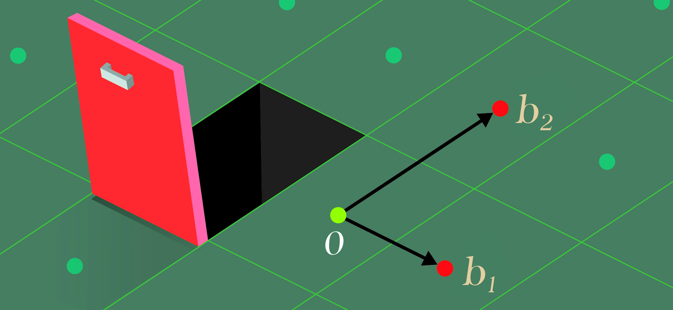
One of the most fascinating things about cryptography is its deeply paradoxical nature: among its early successes is the ability for two strangers to meet, generate a shared secret key, and thereon communicate privately — all of these performed entirely within a crowd. Over the last several decades, we have witnessed ever more surprising cryptographic protocols, achieving increasingly paradoxical properties, ranging from zero knowledge to fully homomorphic encryption. This article will focus on one such paradox, a new technical approach that has been unraveling surprising power, opening up avenues for hitherto unrealized cryptography. This is the unlikely friendship of two seemingly disparate mathematical structures and conjectured hard problems on these, namely, the hardness of finding short independent vectors in high-dimensional lattices and hardness assumptions on elliptic curves over finite fields. This topic is connected with what was explored during the Simons Institute’s Spring 2020 program on Lattices: Algorithms, Complexity, and Cryptography — the interface of lattices with other mathematical structures and new cryptography that can emerge from it.

In more detail, our first assumption on high-dimensional lattices is the so-called learning with errors (LWE) proposed by Oded Regev in 2005 [21]. LWE conjectures that it is hard to recover a secret \(\mathbf{s}\in \mathbb{Z}_q^n\) from a sequence of noisy linear equations on \(\mathbf{s}\). In more detail, given a large prime \(q\) and polynomially many pairs \((\mathbf{a}_i, \langle \mathbf{a}_i,\;\mathbf{s}\rangle + e_i)\), where \(\mathbf{a}_i \in \mathbb{Z}_q^n\) are random and \(e_i \in \mathbb{Z}_q\) are “small” perturbations chosen from some appropriate distribution, the LWE problem asks to find \(\mathbf{s}\). For our second assumption, we require three cyclic groups of large prime order (\(q\), say), \(\mathbb{G}_1\), \(\mathbb{G}_2\), and \(\mathbb{G}_T\). Let \(e:\mathbb{G}_1\times \mathbb{G}_2 \to \mathbb{G}_T\) be a nondegenerate bilinear map or “pairing,” and \(g_1\) and \(g_2\) be the generators of \(\mathbb{G}_1\) and \(\mathbb{G}_2\), respectively. Then, by the bilinearity of the pairing, we have that \(e (\;g_1^a, \; g_2^b \;) = e(\;g_1,\; g_2\;)^{ab}\) for any \(a, b \in \mathbb{Z}_q\). We require that the group operations in \(\mathbb{G}_1\), \(\mathbb{G}_2\), and \(\mathbb{G}_T\) as well as the bilinear map \(e\) can be efficiently computed. In terms of hardness, we will roughly assume that the only information the adversary can learn is via legitimate group and pairing computations on the elements she receives. This strong security guarantee can be formalized in the so-called generic group model [22, 20]. We may think of \(a\) as a secret “message” that is encoded in the exponent of a group element \(g_1^a\). Both LWE and bilinear map–based assumptions have been studied extensively, and we have significant confidence in their hardness. These are also two of the most versatile tools in cryptography and have been used to construct breakthrough applications such as identity-based encryption [5], fully homomorphic encryption [14], and such others. Traditionally, these assumptions were used in mutual exclusion for any given construction, but recently we are learning to combine them in novel non-black-box ways to yield surprising results. In this article, I will describe a recent construction of the primitive of broadcast encryption in a joint work with Shota Yamada [2] where we leveraged a serendipitous interplay of these structures to obtain optimal parameters.

This is the third and last entry in a series of posts about lattice block reduction. See here and here for the first and second parts, resp. In this post I will assume you have read the other parts.

In the first two parts we looked at BKZ and Slide reduction, the former being the oldest and most useful in practice, while the latter achieves the best provable bounds and has the cleaner analysis. While BKZ is a natural generalization of LLL, we have seen that the analysis of LLL does not generalize well to BKZ. One can view Slide reduction as a different generalization of LLL with the goal of also naturally generalizing its analysis. As we mentioned in the first part, there is another analysis technique based on dynamical systems, introduced in [HPS11]. Unfortunately, as applied to BKZ, there are some cumbersome technicalities and the resulting bounds on the output quality are not as tight as we would like them to be (i.e. as for Slide reduction). One can view the algorithm we are considering today – SDBKZ [MW16] – as a generalization of LLL that lends itself much easier to this dynamical systems analysis: it is simpler, cleaner and yields better results. Since part of the goal of today’s post is to demonstrate this very useful analysis technique, SDBKZ is a natural candidate.

SDBKZ

Recall the two tools we’ve been relying on in the first two algorithms, SVP and DSVP reduction of projected subblocks:

We will use both of them again today. Like BKZ, a tour of SDBKZ starts by calling the SVP oracle on successive blocks of our basis. However, when we reach the end of the basis, we will not decrease the size of the window, since this is actually quite inconvenient for the analysis. Instead, we will keep the size of the window constant but switch to DSVP reduction, i.e. at the end of the BKZ tour we DSVP reduce the last block. This will locally maximize the last GSO vector in the basis, just as the first SVP call locally minimized the first vector of the basis. Then we will move the window successively backwards, mirroring a BKZ tour, but using DSVP reduction, until we reach the beginning of the basis again. At this point, we switch back to SVP reduction and move the window forward, etc. So SDBKZ runs in forward and backward tours.

A nice observation here is that the backward tour can be viewed equivalently as: 1) compute the reversed dual basis (i.e. the dual basis with reversed columns), 2) run a forward tour, 3) compute the primal basis again. The first of these two steps is self-inverse: computing the reversed dual basis of the reversed dual basis yields the original primal basis. This means step 3) is actually the same as step 1). So in effect, one can view SDBKZ as simply repeating the following two steps: 1) run a forward tour, 2) compute the reversed dual basis. So it doesn’t matter if we use the primal or the dual basis as input, the operations of the algorithm are the same. This is why it is called Self-Dual BKZ.

There is one caveat with this algorithm: it is not clear, when one should terminate. In BKZ and Slide reduction one can formulate clear criteria, when the algorithm makes no more progress anymore. In SDBKZ this is not the case, but the analysis will show that we can bound the number of required tours ahead of time.

The Analysis

We will start by analyzing the effect of a forward tour. Let \({\mathbf{B}}\) be our input basis. The first call to the SVP oracle in a forward tour replaces \({\mathbf{b}}_1\) with the shortest vector in \({\mathbf{B}}_{[1,k]}\). This means that the new basis \({\mathbf{B}}’\) satifies \(\| {\mathbf{b}}_1′ \| \leq \sqrt{\gamma_k} (\prod_{i=1}^k \|{\mathbf{b}}_i^* \|)^{1/k}\) by Minkowski’s bound. Equivalently, this can be written as \[\log \| {\mathbf{b}}_1′ \| \leq \log \sqrt{\gamma_k} + \frac1k (\sum_{i=1}^k \log \|{\mathbf{b}}_i^* \|).\] So if we consider the \(\log \|{\mathbf{b}}_i^*\|\) as variables, it seems like linear algebra could be useful here. So far, so good. The second step is more tricky though. We know that the next basis \({\mathbf{B}}”\), i.e. after the call to the SVP oracle on \({\mathbf{B}}’_{[2,k+1]}\), satisfies \({\mathbf{b}}_1” = {\mathbf{b}}_1’\) and \(\| ({\mathbf{b}}_2”)^* \| \leq \sqrt{\gamma_k} (\prod_{i=2}^{k+1} \|({\mathbf{b}}’_i)^* \|)^{1/k}\). Unfortunately, we have no control over \(\|({\mathbf{b}}’_i)^* \|\) for \(i \in {2,\dots,k} \), since we do not know how the SVP oracle in the first call changed these vector. However, we do know that the lattice \({\mathbf{B}}_{[1,k+1]}\) did not change in that call. So we can write \[\prod_{i=2}^{k+1} \|({\mathbf{b}}’_i)^* \| = \frac{\prod_{i=1}^{k+1} \|{\mathbf{b}}_i^* \|}{\| {\mathbf{b}}’_1 \|}\] and thus we obtain \[\log \| ({\mathbf{b}}_2′)^* \| \leq \log \sqrt{\gamma_k} + \frac1k (\sum_{i=1}^{k+1} \log \|{\mathbf{b}}_i^* \| – \log \|{\mathbf{b}}’_1 \|).\] Again, this looks fairly “linear algebraicy”, so it could be useful. But there is another issue now: in order to get an inequality purely in the input basis \({\mathbf{B}}\), we would like to use our inequality for \(\log \|{\mathbf{b}}_1′ \|\) in the one for \(\log \| ({\mathbf{b}}_2′)^* \|\). But the coefficient of \(\log \|{\mathbf{b}}_1′ \|\) is negative, so we would need a lower bound for \(\log \|{\mathbf{b}}_1′ \|\). Furthermore, we would like to use upper bounds for our variables later, since the analysis of a tour will result in upper bounds and we would like to apply it iteratively. For this, negative coefficients are a problem. So, we need one more modification: we will use a change of variable to fix this. Instead of considering the variables \(\log \| {\mathbf{b}}_i^* \|\), we let the input variables to our forward tour be \(x_i = \sum_{j < k+i} \log \|{\mathbf{b}}^*_i \|\) and the output variables \(y_i = \sum_{j \leq i} \log \|({\mathbf{b}}’_i)^* \|\) for \(i \in [1,\dots,n-k]\). Clearly, we can now write our upper bound on \(\log \|({\mathbf{b}}’_1)^*\|\) as \[y_1 \leq \log \sqrt{\gamma_k} + \frac{x_1}{k}.\] More generally, we have \[\|({\mathbf{b}}’_i)^* \| \leq \sqrt{\gamma_k} \left(\frac{\prod_{j=1}^{i+k-1} \|{\mathbf{b}}_j^* \|}{\prod_{j=1}^{i-1} \|({\mathbf{b}}’_j)^* \|} \right)^{\frac1k}\] which means for our variables \(x_i\) and \(y_i\) that \[y_i = y_{i-1} + \log \| ({\mathbf{b}}’_i)^* \| \leq y_{i-1} + \log \sqrt{\gamma_k} + \frac{x_i – y_{i-1}}{k} = (1-\frac1k) y_{i-1} + \frac1k x_i + \log \sqrt{\gamma_k}.\]

Note that we can write each \(y_i\) in terms of \(x_i\) and the previous \(y_i\) with only positive coefficients. So now we can apply induction to write each \(y_i\) only in terms of the \(x_i\)’s, which shows that \[y_i = \frac1k \sum_{j=1}^i \omega^{i-j} x_j + (1-\omega)^i k \alpha\] where we simplified notation a little by defining \(\alpha = \log \sqrt{\gamma_k}\) and \(\omega = 1-\frac1k\). By collecting the \(x_i\)’s and \(y_i\)’s in a vector each, we have the vectorial inequality \[{\mathbf{y}} \leq {\mathbf{A}} {\mathbf{x}} + {\mathbf{b}}\] where \[{\mathbf{b}} = \alpha k \left[ \begin{array}{c} 1 – \omega \\ \vdots \\ 1 – \omega^{n-k} \end{array}\right] \qquad\qquad {\mathbf{A}} = \frac1k \left[ \begin{array}{cccc} 1 & & & \\ \omega & 1 & & \\ \vdots & \ddots & \ddots & \\ \omega^{n-k-1} & \cdots & \omega & 1 \end{array} \right].\]

Now recall that after a forward tour, SDBKZ computes the reversed dual basis. Given the close relationship between the primal and the dual basis and their GSO, one can show that simply reversing the vector \({\mathbf{y}}\) will yield the right variables \({\mathbf{x}}’_i\) to start the next “forward tour” (which is actually a backward tour, but on the dual). I.e. after reversing \({\mathbf{y}}\), the variables represent the logarithm of the corresponding subdeterminants of the dual basis. (For this we assume for convenience and w.l.o.g. that the lattice has determinant 1; otherwise, there would be a scaling factor involved in this transformation.)

In summary, the effect on the vector \({\mathbf{x}}\) of executing once the two steps, 1) forward tour and 2) computing the reversed dual basis, can be described as \[{\mathbf{x}}’ \leq {\mathbf{R}} {\mathbf{A}} {\mathbf{x}} + {\mathbf{R}} {\mathbf{b}}\] where \({\mathbf{R}}\) is the reversed identity matrix (i.e. the identity matrix with reversed columns). Iterating the two steps simply means we will be iterating the vectorial inequality above. So analyzing the affine dynamical system \[{\mathbf{x}} \mapsto {\mathbf{R}} {\mathbf{A}} {\mathbf{x}} + {\mathbf{R}} {\mathbf{b}}\] will allow us to deduce information about the basis after a certain number of iterations.

Small Digression: Affine Dynamical Systems

Consider some dynamical system \({\mathbf{x}} \mapsto {\mathbf{A}} {\mathbf{x}} + {\mathbf{b}} \) and assume it has exactly one fixed point, i.e. \({\mathbf{x}}^*\) such that \({\mathbf{A}} {\mathbf{x}}^* + {\mathbf{b}} = {\mathbf{x}}^* \). We can write any input \({\mathbf{x}}’\) as \({\mathbf{x}}’ = {\mathbf{x}}^* + {\mathbf{e}}\) for some “error vector” \({\mathbf{e}}\). When applying the system to it, we get \({\mathbf{x}}’ \mapsto {\mathbf{A}} {\mathbf{x}}’ + {\mathbf{b}} = {\mathbf{x}}^* + {\mathbf{A}} {\mathbf{e}}\). So the error vector \({\mathbf{e}}\) is mapped to \({\mathbf{A}} {\mathbf{e}}\). Applying this \(t\) times maps \({\mathbf{e}}\) to \({\mathbf{A}}^t {\mathbf{e}}\), which means after \(t\) iterations the error vector has norm \(\|{\mathbf{A}}^t {\mathbf{e}} \|_{p} \leq \|{\mathbf{A}}^t \|_{p} \| {\mathbf{e}} \|_{p} \) (where \(\| \cdot \|_{p}\) is the matrix norm induced by the vector \(p\)-norm). If we can show that \(\|{\mathbf{A}} \|_p \leq 1 – \epsilon\), then \(\|{\mathbf{A}}^t \|_p \leq \|A \|^t \leq (1-\epsilon)^t \leq e^{-\epsilon t}\), so the error vector will decay exponentially in \(t\) with base \(e^{-\epsilon}\) and the algorithm converges to the fixed point \({\mathbf{x}}^*\).

Back to our concrete system above. As we just saw, we can analyze its output quality by computing its fixed point and its running time by computing \(\|{\mathbf{R}} {\mathbf{A}} \|_p\) for some induced matrix \(p\)-norm. Since this has been a lenghty post already, I hope you’ll trust me that our system above has a fixed point \({\mathbf{x}}^*\), which can be written out explicitely in closed form. As a teaser, its first coordinate is \[x^*_1 = \frac{(n-k)k}{k-1} \alpha.\] This means that if the algorithm converges, it will converge to a basis such that \(\sum_{j \leq k}\log \| {\mathbf{b}}_j^*\| \leq \frac{(n-k)k}{k-1} \log \sqrt{\gamma_k}\). Applying Minkowski’s Theorem to the first block \({\mathbf{B}}_{[1,k]}\) now shows that the shortest vector in this block satisfies \(\lambda_1({\mathbf{B}}_{[1,k]}) \leq \sqrt{\gamma_k}^{\frac{n-1}{k-1}}\). Note that the next forward tour will find a vector of such length. Recall that we assumed that our lattice has determinant 1, so this is exactly the Hermite factor achieved by Slide reduction, but for arbitrary block size (we do not need to assume that \(k\) divides \(n\)) and better than what we can achieve for BKZ (even using the same technique). Moreover, the fixed point actually gives us more information: the other coordinates (that I have ommited here) allow us control over all but \(k\) GSO vectors and by terminating the algorithm at different positions, it allows us to choose which vectors we want control over.

It remains to show that the algorithm actually converges and figure out how fast. It is fairly straight-forward to show that \[\|{\mathbf{R}} {\mathbf{A}}\|_{\infty} = \|{\mathbf{A}}\|_{\infty} = 1 – \omega^{n-k} \approx e^{-\frac{n-k}{k}}.\] (Consider the last row of \({\mathbf{A}}\).) This is always smaller than 1, so the algorithm does indeed converge. For \(k = \Omega(n)\) this is bounded far enough from 1 such that the system will converge to the fixed point up to an arbitrary constant in a number of SVP calls that is polynomial in \(n\). Using another change of variable [N16] or considering the relative error instead of the absolute error [MW15], one can show that this also holds for smaller \(k\).

As mentioned before, this type of analysis was introduced in [HPS11] and has inspired new ideas even in the heuristic analysis of BKZ. In particular, one can predict the behavior of BKZ by simply running such a dynamical system on typical inputs (and making some heuristic assumptions). This idea has been and is being used extensively in cryptanalysis and in optimizing parameters of state-of-the-art algorithms.

Finally, a few last words on SDBKZ: we have seen that it achieves a good Hermite factor, but what can we say about the approximation factor? I actually do not know if the algorithm achieves a good approximation factor and also do not see a good way to analyze it. However, there is a reduction [L86] from achieving approximation factor \(\alpha\) to achieving Hermite factor \(\sqrt{\alpha}\). So SDBKZ can be used to achieve approximation factor \(\gamma_k^{\frac{n-1}{k-1}}\). This is a little unsatisfactory in two ways: 1) the reduction results in a different algorithm, and 2) the bound is a little worse than the factor achieved by slide reduction, which is \(\gamma_k^{\frac{n-k}{k-1}}\). On a positive note, a recent work [ALNS20] has shown that, due to the strong bound on the Hermite factor, SDBKZ can be used to generalize Slide reduction to arbitrary block size \(k\) in a way to achieve the approximation factor \(\gamma_k^{\frac{n-k}{k-1}}\). Another recent work [ABFKSW20] exploited the fact that SDBKZ allows to heuristically predict large parts of the basis to achieve better bounds on the running time of the SVP oracle.

• Lovász. An Algorithmic Theory of Numbers, Graphs and Convexity. 1986

• Hanrot, Pujol, Stehlé. Analyzing blockwise lattice algorithms using dynamical systems. CRYPTO 2011

• Micciancio, Walter. Practical, predictable lattice basis reduction – Full Version. http://eprint.iacr.org/2015/1123

• Micciancio, Walter. Practical, predictable lattice basis reduction. EUROCRYPT 2016

• Neumaier. Bounding basis reduction properties. Designs, Codes and Cryptography 2016

• Aggarwal, Li, Nguyen, Stephens-Davidowitz. Slide Reduction, Revisited—Filling the Gaps in SVP Approximation. CRYPTO 2020

• Albrecht, Bai, Fouque, Kirchner, Stehlé, Wen. Faster Enumeration-based Lattice Reduction: Root Hermite Factor \(k^{(1/(2k))}\) in Time \(k^{(k/8 + o(k))}\). CRYPTO 2020

by Siobhan Roberts (Journalist in Residence, Simons Institute)

In January 2014, during an open problems session in the auditorium at the Simons Institute, the computer scientist Thomas Vidick posed a question that he expected would go nowhere.

The research program on Quantum Hamiltonian Complexity had just commenced — probing techniques from both quantum complexity theory and condensed matter physics and asking questions such as: Is the scientific method sufficiently powerful to understand general quantum systems? Is materials science about to hit a computational barrier? 

Vidick’s questions waded further into the weeds. 

“A central conjecture, the so-called quantum PCP conjecture, crystallizes many of these issues, and the conjecture was hotly debated throughout the semester,” recounted Vidick, a professor of computing and mathematical sciences at Caltech, in his research vignette published later that year.

Two of the program’s organizers, Umesh Vazirani of UC Berkeley and Dorit Aharonov at the Hebrew University of Jerusalem, encouraged him to formulate a new variant of the conjecture, which (for those readers at least somewhat in the know) he described as follows:

“This formulation of the PCP theorem gives rise to a quantum analogue whose relation to the quantum PCP conjecture is a priori unclear. The new variant asks the following: Do all languages in QMA admit an efficient verification procedure of the above form, in which the verifier and communication may be quantum? Here it is important to also allow the provers to be initialized in an arbitrary entangled state, as this may be necessary to encode the QMA witness whose existence the provers are supposed to convey to the verifier.”

Vidick admitted the problem was tantalizing, yet he believed it would lead to a dead end.

Six years later, however, quite the contrary has proved to be the case: that dead-end question ultimately led to a breakthrough result.

The day before the 2020 spring term began at the Simons Institute — with a timely pairing of two interconnected programs, Lattices: Algorithms, Complexity, and Cryptography and The Quantum Wave in Computing — Vidick and his collaborators¹ posted a 165-page paper to arXiv titled “MIP*=RE.”

It had been a long time coming. And during the home stretch, another team of researchers seemed to have proved the opposite result — via a very different language and approach — but a gap emerged with a lemma that could not be fixed.

by Prasad Raghavendra

Amid the biggest pandemic in a century, one that has disrupted lives and livelihoods the world over, it is gratifying to see how people in different walks of life have found ways to cope and carry on. Within the realm of theory research, the pursuit to better understand the foundations of computation and their implications doesn’t seem to have slowed down even a bit.

Make no mistake, the pandemic has disrupted our traditional modes of operation. A typical theorist might spend several hours each day brainstorming in a group, often over a beverage. For most theorists, this is the single most productive and enjoyable activity each day. As these meetings move online, they remain a shadow of what they used to be. Normally, surprising results often arise out of chance encounters between researchers from very different areas. As conferences and workshops shift online, however, these chance encounters become very rare. Finally, on most days, we are struggling along an unforgiving trail in an attempt to scale a seemingly insurmountable peak. Doubts — such as, Are we on the right trail? Even if we are on the right trail, are we strong enough to get through it? — often linger and can easily set one up for failure. Sharing these “theoretical” struggles with other researchers over lunch or in the corridors can be critical to keep us going. Sadly, these opportunities are rare these days.

Yet theory research does not seem to have missed a beat. The ACM STOC conference was held online for the first time. Despite the limitations of the medium, there are many silver linings to an online conference. Participation at the conference nearly doubled from last year, with 606 participants from 33 countries, many of which had not been represented at typical STOC conferences before. The videos of the conference talks are all available online, a fantastic resource for researchers going forward. Finally, as Ronen Eldan’s talk at the conference beautifully demonstrated, video is a really effective medium to communicate a research work in broad strokes in a very short time. In fact, this year’s online conference seemed to have so many advantages that the PC chair, Julia Chuzhoy, suggested holding the STOC conference twice each year, once online and once offline. 

As weekly seminars at most universities move online, they have begun to attract participants from across the world. CS Theory Online Talks maintains a list of theory talks that are available online (also see here and here). The PIMS-CRM summer school on probability has morphed into a great set of online courses that I have really enjoyed. The Oxford-Warwick Complexity Meetings are an online lecture series dedicated to complexity theory, while we at the Simons Institute are also hosting a lecture series, on Boolean function analysis (more on this later). This flurry of online activity catalyzed by the pandemic is promising to make theory research broadly accessible to graduate students and undergraduates across the globe.

Meanwhile, fantastic new results keep pouring in. The biggest breakthrough this summer is the work of Karlin, Klein, and Oveis Gharan on the metric traveling salesman problem (metric TSP). They have posted a 1.5 – ε approximation algorithm for metric TSP for some constant ε > 10 ^-36. Metric TSP is a fundamental combinatorial optimization problem wherein the inputs consist of a network of cities and the distances between them. The goal is to find the shortest-length route that visits each city exactly once and returns to the starting point. This problem is called metric TSP if the distances between cities are assumed to satisfy the triangle inequality, namely the distance from City A to City C is at most the sum of the distances from City A to City B and from City B to City C. 

by Daniel Hsu

The practice of deep learning has attracted new attention to several basic questions in statistical machine learning. One such question is how fitting machine learning models to relatively small “training” data sets can lead to accurate predictions on new data. In machine learning jargon, this is the question of generalization.

The conventional wisdom in machine learning offers the following about generalization:

1. A model that is too simple will underfit the true patterns in the training data, and thus, it will predict poorly on new data.
2. A model that is too complicated will overfit spurious patterns in the training data; such a model will also predict poorly on new data.

Consequently, one should choose a model that balances these concerns of underfitting and overfitting [30]. A textbook corollary is that a model that exactly fits — i.e., interpolates — the training data “is overfit to the training data and will typically generalize poorly” [17].

Recent machine learning practice appears to eschew this conventional wisdom in a dramatic fashion. For instance, a common starting point for training a neural network is to find a model that exactly fits the training data [27]. (Typically, the model is subsequently fine-tuned using different criteria, but the starting point is already nontrivial.) While this may be difficult or impossible with small neural networks, it becomes substantially easier after making the network very large. It is remarkable that this practice is compatible with generalization, despite the concerns about overfitting.

This apparent contradiction of conventional wisdom is not new. In the last century, machine learning practitioners were already aware of the efficacy (and advantages) of using “oversized” neural networks where the number of model parameters exceeds the number of training data [9, 20]. Similar observations were made about large ensembles of decision trees: it was found that increasing the number of decision trees in an ensemble could improve accuracy, even beyond the point at which the ensemble exactly fit the training data [28]. These empirical observations motivated the development of a new theory that greatly sharpens the existing body of knowledge in statistical machine learning [1, 28], and this theory has been recently extended to deep neural networks [2, 15, 26].

However, the new theory does not fully explain recent observations about interpolating neural networks. First, in more recent experiments, neural networks are trained to interpolate noisy data [34]. By noisy data, we mean data in which the prediction targets (labels) may be erroneous. In fact, experiments have been conducted in which noise is deliberately injected in the data by assigning random labels to subsets of the training data. Neural networks that interpolate these data were nevertheless found to have nontrivial accuracy on new data. Second, similar phenomena have been observed in the context of predicting real numerical targets. (The aforementioned theoretical and empirical studies mostly focused on classification targets.) When predicting real numbers, it is almost always a given that training data will have noisy labels, so the thought of interpolating training data seems even more preposterous. But again, in recent experimental studies, interpolating (or nearly interpolating) models were found to have nontrivially accurate predictions on new data [4, 7].

by Prahladh Harsha

An emerging theme in several disciplines of science over the last few decades is the study of local-to-global phenomena. Let me elucidate with a few examples. In biology, one tries to understand the global properties of an organism by studying local interactions at a cellular level. The Internet graph is impossible to predict or control at a global level; what one can at best do is understand its behavior by making changes at a very local level. Moving to examples closer to theoretical computer science, the pioneering works in computation theory due to Turing and others define the computation of any global function as one that can be broken down into a sequence of local computations. The seminal work on NP-completeness due to Cook, Levin, and Karp demonstrates that any verification task can be in fact reduced to a conjunction of verifying very local objects.

Given these examples, an intriguing question that arises in multiple disciplines is to identify which objects support such local-to-global phenomena. This question as stated is an ill-formed one, but one can attempt to make it well-defined in a variety of contexts. Let me illustrate by giving three specific instances.

Mixing time in graphs: Which graphs have the property of having a global mixing property that can be inferred by understanding the mixing properties of several related smaller graphs?

Local testing and decoding (in coding theory): Which error-correcting codes have the property of being able to be tested or decoded by looking at the code word or received word very locally (i.e., at very few locations)?

Topologically expanding graphs: Which graphs or hypergraphs have the property that their global topological property can be inferred by their local topological behavior?

These questions, seemingly disparate and arising in very different contexts and communities (in particular, approximate sampling, coding theory, and topology), surprisingly all led to the investigation of a similar expanding object: the high-dimensional expander. The Simons Institute 2019 summer cluster on Error-Correcting Codes and High-Dimensional Expansion brought together researchers from these diverse communities to study high-dimensional expanders and their potential applications to mathematics and theoretical computer science.

What is a high-dimensional expander?

High-dimensional expanders (HDXs) are a high-dimensional analogue of expander graphs. An expander graph, loosely speaking, is an extremely well-connected graph. Analytically, this is best captured via the second-largest eigenvalue (in absolute value) of the normalized adjacency matrix of the graph. More precisely, a graph G is said to be a λ-expander (for λ ∈ [0,1]) if the second-largest eigenvalue (in absolute value) of the normalized adjacency matrix A_G of G is bounded above by λ. The smaller the λ, the better the expander. An equivalent definition is in terms of how well the random walk on the vertices induced by the graph mixes: G is a λ-expander if the spectral norm of the difference of the normalized adjacency matrix A_G and the normalized all-ones matrix J (the normalized adjacency matrix of the complete graph) is bounded above by λ (i.e., \[\left\| A_G – \frac1n J \right\| \leq \lambda,\]

where n is the number of vertices of the graph G).

by Shayan Oveis Gharan

Classical theorems in theoretical computer science typically heavily exploit combinatorial or probabilistic tools. Later on, linear algebraic and geometric tools proved to be fundamental elements in numerous algorithmic or hardness results. In this research vignette, I will explain a new tool known as the “polynomial paradigm,” which can be seen as a bridge between linear algebraic and probabilistic methods; and I will discuss some unexpected applications in computer science. 

Given a polynomial \(p \in R\lbrack z_{1},\ldots,z_{n}\rbrack\), we can think of it in three ways: (i) coefficients of p, (ii) zeros of p, or (iii) a function that maps n-dimensional complex vectors to complex numbers. Having these three different representations, one can study what happens to one representation when we change another one, or what happens when we apply a mathematical operation such as differentiation, integration, or specialization. For many years, mathematicians studied these questions for many classes of polynomials.

Over the last two decades, a new theme that we call the “polynomial paradigm” emerged. It was observed that if the roots of the (multivariate) polynomial \(p\) have a “nice” structure in the n-dimensional complex plane, then one can study the interaction of zeros, coefficients, and function values rigorously. In several pioneering works, Borcea, Brändén, Choe, Liggett, Oxley, Sokal, and Wagner studied the class of real stable polynomials, which can be seen as the right multivariate generalization of real-rooted polynomials. A polynomial \(p\) is real stable if it has no root in the upper half of the n-dimensional complex plane. They observed that this class is closed under many operations, such as specialization, differentiation, inversion, etc.

Over the last decade, the polynomial paradigm proved to be a fruitful approach in many areas of science and mathematics. Several applications of this paradigm in theoretical computer science, combinatorics, and linear algebra were discovered, such as improved approximation algorithms for the traveling salesman problem, a purely algebraic proof of the van der Waerden conjecture, and a resolution of the notorious Kadison-Singer conjecture. The general recipe in almost all these applications is as follows: Given a discrete phenomenon, encode it in a complex multivariate polynomial with a nice zero-free region, such as a real stable polynomial. Then study this polynomial via the interplay of coefficients, zeros, and function values. Finally, translate your findings to the domain of the original problem.

In Spring 2019, with Nikhil Srivastava, we organized a semester-long program on Geometry of Polynomials at the Simons Institute, where we invited researchers across several areas of science, mathematics, and computer science to explore this rapidly evolving area. A large group tried to better understand these polynomials and their properties, while many others tried to explore further applications. In the rest of this research vignette, I will explain the journey toward the discovery of a new class of multivariate polynomials that we call completely log-concave polynomials. This discovery and their application motivated several researchers within the program to start collaborating to better understand this class of polynomials and its properties.

1 Introduction

1.1 Lattices and lattice-based cryptography

Lattices are classically-studied geometric objects that in the past few decades have found a multitude of applications in computer science. The most important application area is lattice-based cryptography, the design of cryptosystems whose security is based on the apparent intractability of computational problems on lattices, even for quantum computers. Indeed, lattice-based cryptography has revolutionized the field because of its apparent quantum resistance and its other attractive security, functionality, and efficiency properties.

Intuitively, a lattice is a regular ordering of points in some (typically high-dimensional) space. More precisely, a lattice \( {{\cal{L}}}\) of rank \( {n}\) is the set of all integer linear combinations of some linearly independent vectors \( {\mathbf{b}_1, \ldots, \mathbf{b}_n}\), which are called a basis of \( {{\cal{L}}}\). We will be primarily interested in analyzing the running times of lattice algorithms as functions of the lattice’s rank \( {n}\).

1.2. Computational lattice problems

The two most important computational problems on lattices are the Shortest Vector Problem (SVP) and the Closest Vector Problem (CVP). SVP asks, given a basis of a lattice \( {{\cal{L}}}\) as input, to find a shortest non-zero vector in \( {{\cal{L}}}\). CVP, which can be viewed as an inhomogeneous version of SVP, asks, given a basis of a lattice \( {{\cal{L}}}\) and a target point \( {\mathbf{t}}\) as input, to find a closest vector in \( {{\cal{L}}}\) to \( {\mathbf{t}}\).

Algorithms for solving SVP form the core of the best known attacks on lattice-based cryptography both in theory and in practice. Accordingly, it is critical to understand the precise complexity of SVP as well as possible. The best provably correct algorithms for both SVP and CVP run in \( {2^{n + o(n)}}\)-time [ADRS15, ADS15, AS18a]. The best heuristic algorithms for SVP run in \( {2^{cn + o(n)}}\)-time for \( {c = 0.292}\) classically [BDGL16] and \( {c = 0.265}\) using quantum speedups [Laa15] (see also [KMPR19]), and most real-world lattice-based cryptosystems assume that these algorithms are close to optimal. Indeed, many of these cryptosystems assume what Bos et al. [B+16] call a “paranoid” worst-case estimate of \( {c = 0.2075}\) (based on the kissing number and assuming that sieving algorithms are optimal) as the fastest hypothetical running time for SVP algorithms when choosing parameters. (See also Albrecht et al. [A+18], which surveys the security assumptions made in a wide range of lattice-based cryptosystems.) Accordingly, the difference in being able to solve SVP in \( {2^{0.2075n}}\) versus \( {2^{n/20}}\) versus \( {2^{\sqrt{n}}}\) time may mean the difference between lattice-based cryptosystems being secure, insecure with current parameters, or effectively broken in practice.

There is a rank-preserving reduction from SVP to CVP [GMSS99], so any algorithm for CVP immediately gives an essentially equally fast algorithm for SVP. In other words, CVP is at least as hard as SVP (and probably a bit harder). Indeed, historically, almost all lower bounds for SVP are proven via reduction from CVP (and nearly all algorithmic progress on CVP uses ideas originally developed for SVP).

1.3. Fine-grained hardness

The field of fine-grained complexity works to give strong, quantitative lower bounds on computational problems assuming standard complexity-theoretic assumptions. Proving such a (conditional) lower bound for an \( {{\mathsf{NP}}}\)-hard problem generally works by (1) assuming a stronger hardness assumption than \( {{\mathsf{P}} \neq {\mathsf{NP}}}\) about the complexity of \( {k}\)-SAT (such as ETH or SETH, defined below), and (2) giving a highly efficient reduction from \( {k}\)-SAT to the problem. The most important hardness assumptions for giving lower bounds on \( {{\mathsf{NP}}}\)-hard problems are the Exponential Time Hypothesis (ETH) and the Strong Exponential Time Hypothesis (SETH) of Impagliazzo and Paturi [IP01]. ETH asserts that there is no \( {2^{o(n)}}\)-time algorithm for \( {3}\)-SAT, and SETH asserts that for every \( {\epsilon > 0}\) there exists \( {k \in {\mathbb Z}^+}\) such that there is no \( {2^{(1 – \epsilon)n}}\)-time algorithm for \( {k}\)-SAT, where \( {n}\) denotes the number of variables in the SAT instance.

Here by “highly efficient” reductions we mean linear ones, i.e., reductions that map a \( {3}\)-SAT or \( {k}\)-SAT formula on \( {n}\) variables to an SVP or CVP instance of rank \( {C n + o(n)}\) for some absolute constant \( {C > 0}\). Indeed, by giving a reduction from \( {3}\)-SAT (respectively, \( {k}\)-SAT for any \( {k \in {\mathbb Z}^+}\)) instances on \( {n}\) variables to SVP or CVP instances of rank \( {C n + o(n)}\), we can conclude that there is no \( {2^{o(n)}}\)-time (resp., \( {2^{(1-\epsilon)n/C}}\)-time for any \( {\epsilon > 0}\)) algorithm for the corresponding problem assuming ETH (resp., SETH). Note that the smaller the value of \( {C}\) for which one can show such a reduction, the stronger the conclusion. In particular, a reduction mapping \( {k}\)-SAT instances on \( {n}\) variables to SVP or CVP instances of rank \( {n + o(n)}\) would imply an essentially tight lower bound on the corresponding problem assuming SETH — as mentioned above, the best provably correct algorithms for both SVP and CVP run in time \( {2^{n + o(n)}}\).

1.4. Fine-grained hardness of CVP (and SVP)

It is relatively easy to show that CVP is “ETH-hard,” i.e., to show that a \( {2^{o(n)}}\)-time algorithm for CVP would imply a \( {2^{o(n)}}\)-time algorithm for \( {3}\)-SAT instances with \( {n}\) variables. This would falsify ETH. (It’s a nice exercise to show that the Subset Sum problem on a set of size \( {n}\) reduces to CVP on a lattice of rank \( {n}\), which implies the result.)

With some work, Divesh Aggarwal and Noah extended this to SVP [AS18b]. In particular, we showed a reduction from CVP to SVP that only increases the rank of the lattice by some constant multiplicative factor. (Formally, the reduction only works with certain minor constraints on the CVP instance. The reduction originally relied on a geometric conjecture, which was open for decades. But, Serge Vlăduţ proved the conjecture [Vlă19] shortly after we published!)

So, unless ETH is false, there is no \( {2^{o(n)}}\)-time algorithm for CVP or SVP. But, for cryptographic applications, even, say, a \( {2^{n/20}}\)-time algorithm would be completely devastating. If such an algorithm were found, cryptographic schemes that we currently think are secure against absurdly powerful attackers straight out of science fiction (say, one with a computer the size of the sun running until the heat death of the universe) would turn out to be easily broken (e.g., in seconds on our laptops).

In [BGS17, ABGS20], we almost showed that CVP is “SETH-hard,” i.e., that a \( {2^{(1-\epsilon)n}}\)-time algorithm for CVP would imply such an algorithm for \( {k}\)-SAT for any constant \( {k}\). This would falsify SETH. So, we almost showed that the [ADS15] algorithm is optimal. The “almost” is because our proof works with \( {\ell_p}\) norms, that is, we show hardness for the version of CVP in which the distance from the target to a lattice vector is defined in terms of the \( {\ell_p}\) norm,

\( \displaystyle \|\mathbf{x}\|_p := (|x_1|^p + \cdots + |x_d|^p)^{1/p} \; . \)

We call the corresponding problem \( {{\mathrm{CVP}}_p}\). In fact, our proof works for all \( {\ell_p}\) norms except when \( {p}\) is an even integer. (To see why this might happen, notice \( {\|\mathbf{x}\|_p^p}\) is a polynomial in the \( {x_i}\) if and only if \( {p}\) is an even integer. In fact, there’s some sense in which “\( {\ell_2}\) is the easiest norm,” because for any \( {p}\), there is a linear map \( {A \in {\mathbb R}^{d \times m}}\) such that \( {m}\) is not too large and \( {\|\mathbf{x}\|_2 \approx \|A \mathbf{x}\|_p}\).) Of course, we are most interested in the case \( {p= 2}\) (the only case for which the [ADS15] algorithm works), which is an even integer! Indeed, for all \( {p \neq 2}\), the fastest known algorithm for CVP is still Ravi Kannan’s \( {n^{O(n)}}\)-time algorithm from 1987 [Kan87]. (For SVP and for constant-factor approximate CVP, \(2^{O(n)}\)-time algorithms are known [DPV11].)

In fact, we showed that for \( {p = 2}\), no “natural” reduction can rule out a \( {2^{3n/4}}\)-time algorithm for CVP under SETH. A “natural” reduction is one with a fixed bijection between witnesses. In particular, any “natural” reduction from \( {3}\)-SAT to CVP must reduce to a lattice with rank at least roughly \( {4n/3}\). So, new ideas will be needed to prove stronger hardness of CVP in the \( {\ell_2}\) norm.

2. Open problems

We now discuss some of the problems that we left open in [BGS17, ABGS20]. For simplicity, we ask for specific results (e.g., “prove that problem \( {A}\) is \( {T}\)-hard under hypothesis \( {B}\)“), but of course any similar results would be very interesting (e.g., “\( {A}\) is \( {T’}\)-hard under hypothesis \( {B’}\)“).

2.1. Hardness in the \(\ell_2\) norm

The most obvious question that we left open is, of course, to prove similar \( {2^n}\)-time hardness results for \( {{\mathrm{CVP}}_2}\) (and more generally for \( {{\mathrm{CVP}}_p}\) for even integers \( {p}\)).

Open problem 1. Show that there is no \( {2^{0.99 n}}\)-time algorithm for \( {{\mathrm{CVP}}_2}\) assuming SETH.

Remember that we showed that any proof of such a strong result would have to use an “unnatural” reduction. So, a fundamentally different approach is needed. One potentially promising direction would be to find a Cook reduction, as our limitations only apply to Karp reductions.

Alternatively, one might try for a different result that gets around this “natural” reduction limitations. E.g., even the following much weaker result would be very interesting.

Open problem 2. Show an efficient reduction from \( {3}\)-SAT on \( {n}\) variables to \( {{\mathrm{CVP}}_2}\) on a lattice of rank \( {\approx 10n}\).

Such a reduction to \( {{\mathrm{CVP}}_2}\) on a lattice of rank \( {Cn}\) for some large constant \( {C}\) is known by applying the Sparsification Lemma [IPZ01] to \( {3}\)-SAT, but showing such a reduction for any reasonably small \( {C}\) or even any explicit \( {C}\) using a different proof technique would be interesting.

Also, our limitations only apply to reductions that map satisfying assignments to exact closest vectors. So, one might try to get around our limitation by working directly with approximate versions of \( {3}\)-SAT and \( {{\mathrm{CVP}}_2}\). (In [ABGS20], we show such reductions from Gap-\( {k}\)-SAT to constant-factor approximate \( {{\mathrm{CVP}}_p}\) for all \( {p \notin 2{\mathbb Z}}\) as well as all \( {k \leq p}\). We also show reductions from Gap-\( {k}\)-Parity that achieve relatively large approximation factors.)

Open problem 3. Show an efficient reduction from Gap-\( {3}\)-SAT on \( {n}\) variables to approximate \( {{\mathrm{CVP}}_2}\) on a lattice of rank \( {n}\).

2.2. Hardness in \(\ell_p\) norms

Intuitively, one reason that we are able to prove such strong results for \( {\ell_p}\) norms for \( {p \neq 2}\) is because we can use lattices with large ambient dimension \( {d}\) but low rank \( {n}\). In other words, while our reductions produce lattices \( {{\cal{L}}}\) that live in some \( {n}\)-dimensional subspace of \( {\ell_p}\)-space, the ambient space itself has large dimension \( {d}\) relative to \( {n}\). Of course, any subspace of the \( {\ell_2}\) norm is an \( {\ell_2}\) subspace (i.e., every slice of a ball is a lower-dimensional ball), so in the \( {\ell_2}\) norm, one can assume without loss of generality that \( {d = n}\). In particular, if we were able to prove \( {2^n}\)-hardness for the \( {\ell_2}\) norm, then we would actually prove \( {2^d}\)-hardness for free. However, a potentially easier problem would be to improve the \( {2^n}\)-hardness of \( {{\mathrm{CVP}}_p}\) shown in [BGS17, ABGS20]  to \( {2^d}\)-hardness for some \( p \neq 2 \).

Open problem 4. Show that there is no \( {2^{0.99 d}}\)-time algorithm for \( {{\mathrm{CVP}}_p}\) (for some \( {p}\)) assuming SETH.

More generally, it would be very interesting to settle the fine-grained complexity of \( {{\mathrm{CVP}}_p}\) for some \( {p \neq 2}\) (either in terms of rank \( {n} \) or dimension \( {d} \)). This could take the form either of showing improved algorithms (currently the fastest algorithms for \( {{\mathrm{CVP}}_p}\) for general \( {p}\) run in \( {n^{O(n)}}\)-time [Kan87], and \( {2^{O(n)}}\)-time for a constant approximation factor [DPV11]), or showing super-\( {2^n}\) hardness, or both.

Open problem 5. Show matching upper bounds and lower bounds (under SETH) for \( {{\mathrm{CVP}}_p}\) for some \( {p}\) (possibly with a constant approximation factor).

The case where \( {p = \infty}\) is especially interesting. Indeed, because the kissing number in the \( {\ell_\infty}\) norm is \( {3^n-1}\), one might guess that the fastest algorithms for \( {{\mathrm{CVP}}_\infty}\) and \( {{\mathrm{SVP}}_\infty}\) actually run in time \( {3^{n + o(n)}}\) or perhaps \( {3^{d + o(d)}}\). (See [AM18], which essentially achieves this.) We therefore ask whether stronger lower bounds can be proven in this special case.

Open problem 6. Show that \( {{\mathrm{CVP}}_\infty}\) cannot be solved in time \( {3^{0.99n}}\) (under SETH).

2.3. Hardness closer to crypto

The most relevant problem to cryptography is approximate \( {{\mathrm{SVP}}_2}\) with an approximation factor that is polynomial in the rank \( {n}\). Our fastest algorithms to solve this problem work via a reduction to exact (or near exact) \( {{\mathrm{SVP}}_2}\) with some lower rank \( {n’ = \Theta(n)}\), so that even for these polynomial approximation factors, our fastest algorithms run in time \( {2^{\Omega(n)}}\) (where the hidden constant depends on the polynomial; see Michael’s post for more on this topic). And, hardness results for exact SVP rule out attacks on cryptography that use such reductions. We currently only know how to rule out \( {2^{o(n)}}\)-time algorithms for \( {{\mathrm{SVP}}_2}\) (under the Gap-ETH assumption). We ask whether we can do better. (In [AS18b], we proved the stronger result below for \( {\ell_p}\) norms for large enough \( {p \notin 2{\mathbb Z}}\).)

Open problem 7. Prove that there is no \( {2^{n/10}}\)-time algorithm for \( {{\mathrm{SVP}}_2}\) (under SETH).

Of course, we would ideally like to directly rule out faster algorithms for approximate \( {{\mathrm{SVP}}_2}\) with the approximation factors that are most directly relevant to cryptography. There are serious complexity-theoretic barriers to overcome to get all the way there (e.g., \( {{\mathrm{CVP}}_p}\) and \( {{\mathrm{SVP}}_p}\) are known to be in \( {{\mathsf{NP}}} \cap {{\mathsf{coNP}}}\) for large enough polynomial approximation factors. But, we can still hope to get as close as possible, by proving stronger hardness results for approximate \( {{\mathrm{CVP}}_p}\) and approximate \( {{\mathrm{SVP}}_p}\). Indeed, a beautiful sequence of works showed hardness for approximation factors up to \( {n^{c/\log \log n}}\) (so “nearly polynomial) [DKRS03, HR12], but these results are not fine grained.

The best fine-grained hardness of approximation results known rule out algorithms for small constant-factor approximations for \( {{\mathrm{CVP}}_p}\) with \( {p \notin 2{\mathbb Z}}\) in time \( {2^{0.99n}}\) for \( {{\mathrm{CVP}}_p}\) and \( {{\mathrm{SVP}}_p}\) for any \( {p}\) in time \( {2^{o(n)}}\). We ask whether we can do better.

Open problem 8. Prove that there is no \( {2^{0.99 n}}\)-time algorithm for \( {2}\)-approximate \( {{\mathrm{CVP}}_p}\) (under some form of Gap-SETH, see below).

Open problem 9. Prove that there is no \( {2^{o(n)}}\)-time algorithm for \( {\gamma}\)-approximate \( {{\mathrm{CVP}}_p}\) for superconstant \( {\gamma = \omega(1)}\) (under Gap-ETH).

2.4. Gap-SETH?

One issue that arose in our attempts to prove fine-grained hardness of approximation results is that we don’t even know the “right” complexity-theoretic assumption about approximate CSPs to use as a starting point. For fine-grained hardness of exact problems, ETH and SETH are very well established hypotheses, and they are in some sense “the weakest possible” assumptions of their form. E.g., it is easy to see that \( {k}\)-SAT is \( {2^{Cn}}\) hard if any \( {k}\)-CSP is. But, for hardness of approximation, the situation is less clear.

The analogue of ETH in the regime of hardness of approximation is the beautiful Gap-ETH assumption, which was defined independently by Irit Dinur [Din16] and Pasin Manurangsi and Prasad Raghavendra [MR17]. This assumption says that there exists some constant approximation factor \( {\delta \neq 1}\) such that \( {\delta}\)-Gap-\( {3}\)-SAT cannot be solved in time \( {2^{o(n)}}\). (Formally, both Dinur and Manurangsi and Raghavendra say that there is no \( {2^{o(n)}}\)-time algorithm that distinguishes a satisfiable formula from a formula for which no assignment satisfies more than a \( {(1-\epsilon)}\) fraction of the clauses, but we ignore this requirement of perfect completeness here.) It is easy to see that this hypothesis is equivalent to a similar hypothesis about any \( {3}\)-CSP (or, indeed, any \( {k}\)-CSP for any constant\( {k}\)).

However, to prove hardness of approximation with the finest of grains, we need some “gap” analogue of SETH, i.e., we would like to assume that for large enough \( {k}\), some Gap-\( {k}\)-CSP is hard to approximate up to some constant factor \( {\delta \neq 1}\) in better than \( {2^{0.99n}}\)-time. (Formally, we should add an additional variable \( {\epsilon > 0}\) and have such a hypothesis for every running time \( {2^{(1-\epsilon)n}}\), but we set \( {\epsilon = 0.01}\) here to keep things relatively simple.)

An issue arises here concerning the dependence of the approximation factor \( {\delta}\) on the arity \( {k}\). In particular, recall that \( {k}\)-SAT can be trivially approximated up to a factor of \( {1-2^{-k}}\) (since a random assignment satisfies a \( {1-2^{-k}}\) fraction of the clauses in expectation). So, if we define Gap-SETH in terms of Gap-\( {k}\)-SAT, then we must choose \( {\delta = \delta(k) \geq 1-2^{-k}}\) that converges to one as \(k\) increases. Manurangsi proposed such a version of Gap-SETH in his thesis [Man19, Conjecture 12.1], specifically that for every large enough constant \( {k}\) there exists a constant \( {\delta = \delta(k) \neq 1}\) such that Gap-\( {k}\)-SAT cannot be approximated up to a factor of \( {\delta}\) in time \( {2^{0.99n}}\). (Again, we are leaving out an additional variable, \( {\epsilon}\).)

If we rely on this version of Gap-SETH, then our current techniques seem to get stuck at proving hardness of approximation for, say, \( {\gamma}\)-approximate \( {{\mathrm{CVP}}_p}\) for some non-explicit constant \( {\gamma_p > 1}\) (and, if one works out the numbers, one can see immediately that \( {\gamma_p}\) must be really quite close to one). However, other Gap-\(k\)-CSPs are known to be (\(\mathsf{NP}\)-)hard to approximate up to much better approximation factors. E.g., for any \( {k}\), Gap-\(k\)-Parity is \( {{\mathsf{NP}}}\)-hard to approximate up to any constant approximation factor \( {1/2 < \delta \leq 1}\) [Hås01], and Gap-\( {k}\)-AND is \( {{\mathsf{NP}}}\)-hard to approximate for any constant approximation factor \( {\Omega(k/2^k) \leq \delta \leq 1}\) [Cha16]. Indeed, Gap-\( {k}\)-AND is a quite natural problem to consider in this context since there is a fine-grained, approximation-factor preserving reduction from any Gap-\( {k}\)-CSP to Gap-\( {k}\)-AND. This generality motivates understanding the precise complexity of Gap-\( {k}\)-AND.

Open problem 10. What is the fine-grained complexity of the \( {\delta}\)-Gap-\( {k}\)-AND problem in terms of \( {n}\), \( {k}\), and \( {\delta}\)? In particular, if

\( \displaystyle C_{k,\delta} := \inf \{ C > 0 \ : \ \text{there is a $2^{C_{k,\delta}}$-time algorithm for algorithm for $\delta$-Gap-$k$-AND}\}\)

then what is the behavior of \( {C_{k,\delta}}\) as \( {k \rightarrow \infty}\) (for various functions \( {\delta = \delta(k)}\) of \( {k}\))?

In particular, if one were to hypothesize sufficiently strong hardness of \( {\delta}\)-Gap-\( {k}\)-AND — i.e., to define an appropriate variant of Gap-SETH based on Gap-\( {k}\)-AND — then one might be able to use this hypothesis to prove very strong fine-grained hardness of approximation results. There is a fine-grained (but non-approximation preserving) reduction from Gap-\( {k}\)-AND to Gap-\( {k}\)-SAT, and so Manurangsi’s Gap-SETH is equivalent to the conjecture that there exists some non-explicit \( {\delta(k)}\) such that \( {\lim_{k \rightarrow \infty} C_{k,\delta} = 1}\).

• [ABGS20] Aggarwal, Bennett, Golovnev, Stephens-Davidowitz. Fine-grained hardness of CVP(P)— Everything that we can prove (and nothing else)
• [A+18] Albrecht, Curtis, Deo, Davidson, Player, Postlethwaite, Virdia, Wunderer. Estimate all the {LWE, NTRU} schemes! SCN, 2019.
• [ADRS15] Aggarwal, Dadush, Regev, Stephens-Davidowitz. Solving the Shortest Vector Problem in \(2^n\) time via discrete Gaussian sampling. STOC, 2015.
• [ADS15] Aggarwal, Dadush, Stephens-Davidowitz. Solving the Closest Vector Problem in \(2^n\) time–The discrete Gaussian strikes again! FOCS, 2015.
• [AM18] Aggarwal, Mukhopadhyay. Faster algorithms for SVP and CVP in the \(\ell_\infty\) norm. ISAAC, 2018.
• [AS18a] Aggarwal, Stephens-Davidowitz. Just take the average! An embarrassingly simple \(2^n\)-time algorithm for SVP (and CVP). SOSA, 2018.
• [AS18b] Aggarwal, Stephens-Davidowitz. (Gap/S)ETH hardness of SVP. STOC, 2018.
• [B+16] Bos, Costello, Ducas, Mironov, Naehrig, Nikolaenko, Raghunathan, Stebila. Frodo: Take off the ring! Practical, Quantum-Secure Key Exchange from LWE. CCS, 2016.
• [BDGL16] Becker, Ducas, Gama, Laarhoven. New directions in nearest neighbor searching with applications to lattice sieving. SODA, 2016.
• [BGS17] Bennett, Golovnev, Stephens-Davidowitz. On the quantitative hardness of CVP. FOCS, 2017.
• [Cha16] Chan. Approximation resistance from pairwise-independent subgroups. J. ACM, 2016.
• [Din16] Dinur. Mildly exponential reduction from gap 3SAT to polynomial-gap label-cover.
• [DKRS03] Dinur, Kindler, Raz, Safra. Approximating CVP to within almost-polynomial factors is NP-hard. Combinatorica, 2003.
• [DPV11] Dadush, Peikert, Vempala. Enumerative lattice algorithms in any norm via \(M\)-ellipsoid coverings. FOCS, 2011.
• [GMSS99] Goldreich, Micciancio, Safra, Seifert. Approximating shortest lattice vectors is not harder than approximating closest lattice vectors. IPL, 1999.
• [Hås01] Håstad. Some optimal inapproximability results. J. ACM, 2001.
• [HR12] Haviv, Regev. Tensor-based hardness of the Shortest Vector Problem to within almost polynomial factors. TOC, 2012.
• [IP01] Impagliazzo, Paturi. On the complexity of \(k\)-SAT. JCSS, 2001.
• [IPZ01] Impagliazzo, Paturi, Zane. Which problems have strongly exponential complexity? JCSS, 2001.
• [Laa15] Laarhoven. Search problems in cryptography. Ph.D thesis, 2015.
• [Kan87] Kannan. Minkowski’s convex body theorem and Integer Programming. MOR, 1987.
• [KMPR19] Kirshanova, Mårtensson, Postlethwaite, Roy Moulik. Quantum algorithms for the approximate \(k\)-list problem and their application to lattice sieving. Asiacrypt, 2019.
• [Man19] Manurangsi. Approximation and Hardness: Beyond P and NP.
• [MR17] Manurangsi, Raghavendra. A Birthday Repetition Theorem and Complexity of Approximating Dense CSPs. ICALP, 17.
• [Vlă19] Vlăduţ. Lattices with exponentially large kissing numbers. Moscow J. of Combinatorics and Number Theory, 2019.